Power conservation and complex delay networks

The same techniques will work to analyze any delay network, although for more complicated networks it becomes harder to characterize the results, or to design the network to have specific, desired properties. Another point of view can sometimes be usefully brought to the situation, particularly when flat frequency responses are needed, either in their own right or else to ensure that a complex, recirculating network remains stable at feedback gains close to one.

The central fact we will use is that if any delay network, with either one or many inputs and outputs, is constructed so that its output power (averaged over time) always equals its input power, that network has to have a flat frequency response. This is almost a tautology; if you put in a sinusoid at any frequency on one of the inputs, you will get sinusoids of the same frequency at the outputs, and the sum of the power on all the outputs will equal the power of the input, so the gain, suitably defined, is exactly one.

Figure 7.11: First fundamental building block for unitary delay networks: delay lines in parallel.

In order to work with power-conserving delay networks we will need an explicit definition of ``total average power". If there is only one signal (call it $x[n]$), the average power is given by:

$$P(x[n]) = \left [{{\vert x[0]\vert}^2} + {{\vert x[1]\vert}^2} + \cdots + {{\vert x[N-1]\vert}^2} \right ] / N$$

where $N$ is a large enough number so that any fluctuations in amplitude get averaged out. This definition works as well for complex-valued signals as for real-valued ones. The average total power for several digital audio signals is just the sum of the individual signal's powers:

$$P({x_1}[n] , \ldots , {x_r}[n]) = P({x_1}[n]) + \cdots + P({x_r}[n])$$

where $r$ is the number of signals to be combined.

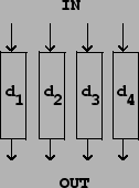
It turns out that a wide range of interesting delay networks has the property that the total power output equals the total power input; they are called unitary. To start with, we can put any number of delays in parallel, as shown in Figure 7.11. Whatever the total power of the inputs, the total power of the outputs has to equal it.

A second family of power-preserving transformations is composed of rotations and reflections of the signals ${x_1}[n]$, ... , ${x_r}[n]$, considering them, at each fixed time point $n$, as the $r$ coordinates of a point in $r$-dimensional space. The rotation or reflection must be one that leaves the origin $(0, \ldots, 0)$ fixed.

For each sample number $n$, the total contribution to the average signal power is proportional to

$${\vert{x_1}\vert}^2 + \cdots + {\vert{x_r}\vert}^2$$

This is just the Pythagorean distance from the origin to the point $({x_1}, \ldots, {x_r})$. Since rotations and reflections are distance-preserving transformations, the distance from the origin before transforming must equal the distance from the origin afterward. So the total power of a collection of signals must must be preserved by rotation.

Figure 7.12: Second fundamental building block for unitary delay networks: rotating two digital audio signals. Part (a) shows the transformation explicitly; (b) shows it as a matrix operation.

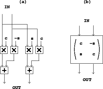Figure 7.12 shows a rotation matrix operating on two signals. In part (a) the transformation is shown explicitly. If the input signals are ${x_1}[n]$ and ${x_2}[n]$, the outputs are:

$${y_1}[n] = c {x_1}[n] - s {x_2}[n]$$

$${y_2}[n] = s {x_1}[n] + c {x_2}[n]$$

where $c, s$ are given by

$$c = \cos(\theta)$$

$$s = \sin(\theta)$$

for an angle of rotation $\theta$. Considered as points on the Cartesian plane, the point $({y_1}, {y_2})$ is just the point $({x_1}, {x_2})$ rotated counter-clockwise by the angle $\theta$. The two points are thus at the same distance from the origin:

$${\vert{y_1}\vert}^2 + {\vert{y_2}\vert}^2 = {\vert{x_1}\vert}^2 + {\vert{x_2}\vert}^2$$

and so the two output signals have the same total power as the two input signals.

For an alternative description of rotation in two dimensions, consider complex numbers $X={x_1} + {x_2}i$ and $Y={y_1} + {y_2}i$. The above transformation amounts to setting

$$Y = XZ$$

where $Z$ is a complex number with unit magnitude and argument $\theta$. Since $\vert Z\vert=1$, it follows that $\vert X\vert = \vert Y\vert$.

If we perform a rotation on a pair of signals and then invert one (but not the other) of them, the result is a reflection. This also preserves total signal power, since we can invert any or all of a collection of signals without changing the total power. In two dimensions, a reflection appears as a transformation of the form

$${y_1}[n] = c {x_1}[n] + s {x_2}[n]$$

$${y_2}[n] = s {x_1}[n] - c {x_2}[n]$$

A special and useful rotation matrix is obtained by setting $\theta = \pi /4$, so that $s = c = \sqrt{1/2}$. This allows us to simplify the computation as shown in Figure 7.13 (part a) because each signal need only be multiplied by the one quantity $c=s$.

Figure 7.13: Details about rotation (and reflection) matrix operations: (a) rotation by the angle $\theta = \pi /4$, so that $a = \cos(\theta) = \sin(\theta) = \sqrt{1/2} \approx 0.7071$; (b) combining two-dimensional rotations to make higher-dimensional ones.

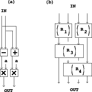More complicated rotations or reflections of more than two input signals may be made by repeatedly rotating and/or reflecting them in pairs. For example, in Figure 7.13 (part b), four signals are combined in pairs, in two successive stages, so that in the end every signal input feeds into all the outputs. We could do the same with eight signals (using three stages) and so on. Furthermore, if we use the special angle $\pi /4$, all the input signals will contribute equally to each of the outputs.

Any combination of delays and rotation matrices, applied in succession to a collection of audio signals, will result in a flat frequency response, since each individual operation does. This already allows us to generate an infinitude of flat-response delay networks, but so far, none of them are recirculating. A third operation, shown in Figure 7.14, allows us to make recirculating networks that still enjoy flat frequency responses.

Figure 7.14: Flat frequency response in recirculating networks: (a) in general, using a rotation matrix $R$; (b) the ``all-pass" configuration.

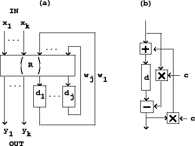Part (a) of the figure shows the general layout. The transformation $R$ is assumed to be any combination of delays and mixing matrices that preserves total power. The signals ${x_1}, \ldots {x_k}$ go into a unitary delay network, and the output signals ${y_1}, \ldots {y_k}$ emerge. Some other signals ${w_1}, \ldots {w_j}$ (where $j$ is not necessarily equal to $k$) appear at the output of the transformation $R$ and are fed back to its input.

If $R$ is indeed power preserving, the total input power (the power of the signals ${x_1}, \ldots {x_k}$ plus that of the signals ${w_1}, \ldots {w_j}$) must equal the output power (the power of the signals ${y_1}, \ldots {y_k}$ plus ${w_1}, \ldots {w_j}$), and subtracting all the $w$ from the equality, we find that the total input and output power are equal.

If we let $j=k=1$ so that there is one $x$, $y$, and $w$, and let the transformation $R$ be a rotation by $\theta$ followed by a delay of $d$ samples on the $W$ output, the result is the well-known all-pass filter. With some juggling, and letting $c = \cos(\theta)$, we can show it is equivalent to the network shown in part (b) of the figure. All-pass filters have many applications, some of which we will visit later in this book.