Fourier analysis and reconstruction of audio signals

Fourier analysis can sometimes be used to resolve the component sinusoids in an audio signal. Even when it can't go that far, it can separate a signal into frequency regions, in the sense that for each $k$, the $k$th point of the Fourier transform would be affected only by components close to the nominal frequency $k\omega$. This suggests many interesting operations we could perform on a signal by taking its Fourier transform, transforming the result, and then reconstructing a new, transformed, signal from the modified transform.

Figure 9.7: Sliding-window analysis and resynthesis of an audio signal using Fourier transforms. In this example the signal is filtered by multiplying the Fourier transform with a desired frequency response.

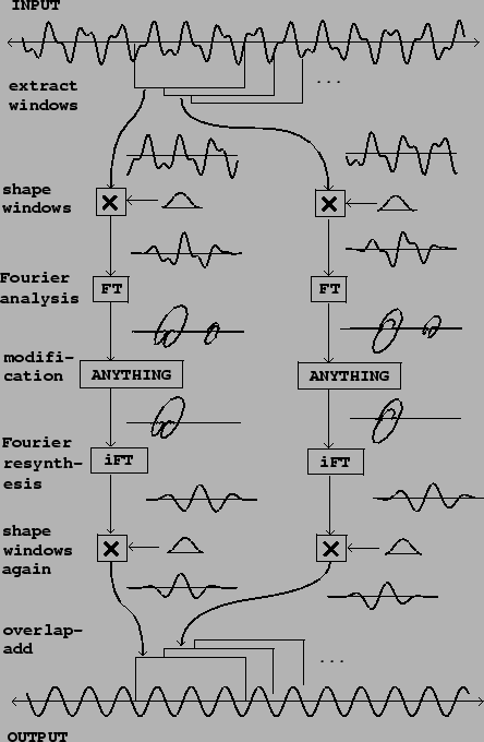Figure 9.7 shows how to carry out a Fourier analysis, modification, and reconstruction of an audio signal. The first step is to divide the signal into windows, which are segments of the signal, of $N$ samples each, usually with some overlap. Each window is then shaped by multiplying it by a windowing function (Hann, for example). Then the Fourier transform is calculated for the $N$ points $k = 0, 1, \ldots, N-1$. (Sometimes it is desirable to calculate the Fourier transform for more points than this, but these $N$ points will suffice here.)

The Fourier analysis gives us a two-dimensional array of complex numbers. Let $H$ denote the hop size, the number of samples each window is advanced past the previous window. Then for each $m = \ldots, 0, 1, \ldots$, the $m$th window consists of the $N$ points starting at the point $mH$. The $n$th point of the $m$th window is $mH+n$. The windowed Fourier transform is thus equal to:

$$S[m, k] = {\cal FT}\{w(n)X[n-mH]\} (k)$$

This is both a function of time ($m$, in units of $H$ samples) and of frequency ($k$, as a multiple of the fundamental frequency $\omega$). Fixing the frame number $m$ and looking at the windowed Fourier transform as a function of $k$:

$$S[k] = S[m, k]$$

gives us a measure of the momentary spectrum of the signal $X[n]$. On the other hand, fixing a frequency $k$ we can look at it as the $k$th channel of an $N$-channel signal:

$$C[m] = S[m, k]$$

From this point of view, the windowed Fourier transform separates the original signal $X[n]$ into $N$ narrow frequency regions, called bands.

Having computed the windowed Fourier transform, we next apply any desired modification. In the figure, the modification is simply to replace the upper half of the spectrum by zero, which gives a highly selective low-pass filter. (Two other possible modifications, narrow-band companding and vocoding, are described in the following sections.)

Finally we reconstruct an output signal. To do this we apply the inverse of the Fourier transform (labeled ``iFT" in the figure). As shown in Section 9.1.2 this can be done by taking another Fourier transform, normalizing, and flipping the result backwards. In case the reconstructed window does not go smoothly to zero at its two ends, we apply the Hann windowing function a second time. Doing this to each successive window of the input, we then add the outputs, using the same overlap as for the analysis.

If we use the Hann window and an overlap of four (that is, choose $N$ a multiple of four and space each window $H=N/4$ samples past the previous one), we can reconstruct the original signal faithfully by omitting the ``modification" step. This is because the iFT undoes the work of the $FT$, and so we are multiplying each window by the Hann function squared. The output is thus the input, times the Hann window function squared, overlap-added by four. An easy check shows that this comes to the constant $3/2$, so the output equals the input times a constant factor.

The ability to reconstruct the input signal exactly is useful because some types of modification may be done by degrees, and so the output can be made to vary smoothly between the input and some transformed version of it.