Butterworth filters

A filter with one real pole and one real zero can be configured as a shelving filter, as a high-pass filter (putting the zero at the point $1$) or as a low-pass filter (putting the zero at $-1$). The frequency responses of these filters are quite blunt; in other words, the transition regions are wide. It is often desirable to get a sharper filter, either shelving, low- or high-pass, whose two bands are flatter and separated by a narrower transition region.

A procedure borrowed from the analog filtering world transforms real, one-pole, one-zero filters to corresponding Butterworth filters, which have narrower transition regions. This procedure is described clearly and elegantly in the last chapter of []. Since it involves passing from the discrete-time to the continuous-time domain, the derivation uses calculus; it also requires using notions of complex exponentiation and roots of unity which we are avoiding here.

To make a Butterworth filter out of a high-pass, low-pass, or shelving filter, suppose that either the pole or the zero is given by the expression

$${{1 - {r^2}} \over {{(1 + r)}^2}}$$

where $r$ is a parameter ranging from 1 to $\inf$. If $r=0$ this is the point $1$, and if $r=\inf$ it's $-1$.

Then, for reasons which will remain mysterious, we replace the point (whether pole or zero) by $n$ points given by:

$${ (1 - {r^2}) - (2 r \sin(\alpha)) i } \over { 1 + {r^2} + 2 r \cos(\alpha))}$$

where $\alpha$ ranges over the values:

$${\pi \over 2} ({1 \over n} - 1) , {\pi \over 2} ({3 \over n} - 1) , \ldots , {\pi \over 2} ({{2n-1} \over n} - 1)$$

In other words, $\alpha$ takes on $n$ equally spaced angles between $-\pi/2$ and $\pi /2$. The points are arranged in the complex plane as shown in Figure 8.17. They lie on a circle through the original real-valued point, which cuts the unit circle at right angles.

A good choice for a nominal cutoff or shelving frequency defined by these circular collections of poles or zeros is simply the spot where the circle intersects the unit circle, corresponding to $\alpha = \pi/2$. This gives the point

$${ (1 - {r^2}) - 2 r i } \over { 1 + {r^2} }$$

which, after some algebra, gives an angular frequency equal to

$$\beta = 2 \arctan (r)$$

Figure 8.17: Replacing a real-valued pole or zero with an array as for a Butterworth filter. In this example we get four new poles or zeros as shown, lying along the circle where $r=0.5$.

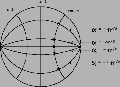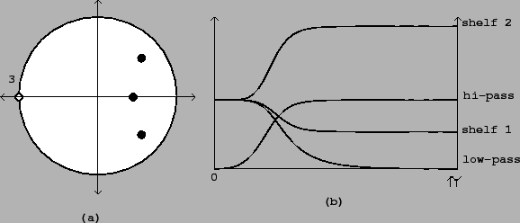
Figure 8.18, part (a), shows a pole-zero diagram and frequency response for a Butterworth low-pass filter with three poles and three zeros. Part (b) shows the frequency response of the low-pass filter and three other filters obtained by choosing different values of $\beta$ (and hence $r$) for the zeros, while leaving the poles stationary. As the zeros progress from $\beta =\pi$ to $\beta =0$, the filter, which starts as a low-pass filter, becomes a shelving filter and then a high-pass one.

Figure 8.18: (a). Pole-zero plot for a Butterworth low-pass filter with three poles and three zeros. The poles are chosen for a cutoff frequency $\beta = \pi /4$. (b). Frequency responses for four filters with the same pole configuration, with different placements of zeros (but leaving the poles fixed). The low-pass filter results from setting $\beta =\pi$ for the zeros; the two shelving filters correspond to $\beta =3\pi /10$ and $\beta =2\pi /10$, and finally the high-pass filter is obtained setting $\beta =0$. The high-pass filter is normalized for unit gain at the Nyquist frequency, and the others for unit gain at DC.