Delay networks

If we consider our digital audio samples $X[n]$ to correspond to successive moments in time, then time shifting the signal by $d$ samples corresponds to a delay of $d/R$ time units, where $R$ is the sample rate. (If $d$ is negative, then we are saying that the output predicts the input; this isn't practical in systems, such as Pd, that schedule computations in order of time.)

Figure 7.3: A delay network. Here we add the incoming signal to a delayed copy of itself.

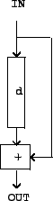
Figure 7.3 shows one example of a linear delay network: an assembly of delay units, possibly with amplitude scaling operations, combined using addition and subtraction. The output is a linear function of the input, in the sense that adding two signals at the input is the same as processing each one separately and adding the results. Moreover, they are time invariant, i.e., they create no new frequencies in the output that weren't present in the input.

In general there are two ways of thinking about delay networks. We can think in the time domain, in which we draw waveforms as functions of time (or of the index $n$), and consider delays as time shifts. Alternatively we may think in the frequency domain, in which we dose the input with a sinusoid (so that its output is a sinusoid at the same frequency) and report the amplitude and/or phase change brought by the network, as a function of the frequency (encoded in the complex number $Z$). We'll now look at the delay network of Figure 7.3 in each of the two ways in turn.

Figure 7.4: The time domain view ot the delay network of Figure 7.3. The output is the sum of the input and its time shifted copy.

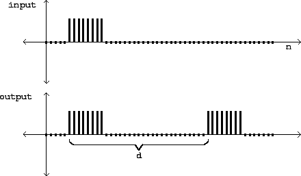Figure 7.4 shows the network's behavior in the time domain. We invent some sort of suitable test function as input (it's a rectangular pulse eight samples wide in this example) and graph the input and output as functions of the sample number $n$. This particular delay network adds the input to a delayed copy of itself.

A frequently used test function is an impulse, which is a pulse lasting only one sample. The utility of this is that, if we know the output of the network for an impulse, we can find the output for any other digital audio signal--because any signal $x[n]$ is a sum of impulses, one of height $x[0]$, the next one occurring one sample later and having height $x[1]$, and so on. Later, when the networks get more complicated, we will move to using impulses as input signals to show their time-domain behavior.

On the other hand, we can analyze the same network in the frequency domain by considering a (complex-valued) test signal,

$$X[n] = {Z^n}$$

where Z has unit magnitude and argument $\omega$. We already know that the output is another complex sinusoid with the same frequency, that is,

$$H {Z^N}$$

for some complex number $H$ (which we want to find.) So we write the output directly as the sum of the input and its delayed copy:

$${Z^n} + {Z^{-d}} {Z^n} = (1 + {Z^{-d}}) {Z^n}$$

and find by inspection that:

$$H = 1 + {Z^{-d}}$$

We can understand the frequency-domain behavior of this delay network by studying how the complex number $H$ varies as a function of the angluar frequency $\omega$. We are especially interested in its argument and magnitude--which tell us the relative phase and amplitude of the sinusoid that comes out. We will work this example out in detail to show how the arithmetic of complex numbers can predict what happens when sinusoids are combined additively.

Figure 7.5: Analysis, in the complex plane, of the frequency-domain behavior of the delay network of Figure 7.3. The complex number $Z$ encodes the frequency of the input. The delay line output is the input times $Z^-d$. The total (complex) gain is $H$. We find the magnitude and argument of $H$ by symmetrizing the sum, rotating it by $d/2$ times the angular frequency of the input.

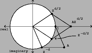Figure 7.5 is a graph, in the complex plane, showing how the quantities $1$ and ${Z^{-d}}$ combine additively. To add complex numbers we add their real and complex parts separately. So the complex number $1$ (real part $1$, imaginary part $0$) is added coordinate-wise to the complex number ${Z^{-d}}$ (real part $\cos(-d \omega)$, imaginary part $\sin(-d \omega)$). This is shown graphically by making a parallelogram, with corners at the origin and at the two points to be added, and whose fourth corner is the sum $H$.

As the figure shows, the result can be understood by symmetrizing it about the real axis: instead of $1$ and ${Z^{-d}}$, it's easier to sum the quantities ${Z^{d/2}}$ and ${Z^{-d/2}}$, because they are symmetric about the real (horizontal) axis. (Strictly speaking, we haven't defined the quantities ${Z^{d/2}}$ and ${Z^{-d/2}}$; we use those expressions to denote unit complex numbers whose arguments are half those of $Z^d$ and $Z^{-d}$.) We rewrite the gain as:

$$H = {Z^{-d/2}} ({Z^{d/2}} + {Z^{-d/2}})$$

The first term is a phase shift of $-d \omega / 2$. The second term is best understood in rectangular form:

$${Z^{d/2}} + {Z^{-d/2}}$$

$$= (\cos(\omega d / 2) + i \sin(\omega d / 2)) + (\cos(\omega d / 2) - i \sin(\omega d / 2))$$

$$= 2 \cos(\omega d / 2)$$

This real-valued quantity may be either positive or negative; its absolute value gives the magnitude of the output:

$$\vert H\vert = 2 \vert\cos(\omega d / 2) \vert$$

The quantity $\vert H\vert$ is called the gain of the delay network at the angular frequency $\omega$, and is graphed in Figure 7.6. The frequency-dependent gain of a delay network (that is, the gain as a function of frequency) is called the network's frequency response.

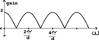
Since the network has greater gain at some frequencies than at others, it may be considered as a filter, that can be used to separate certain components of a sound from others. Because of the shape of this particular gain expression as a function of $\omega$, this kind of delay network is called a (non-recirculating) comb filter.

Figure 7.6: Gain of the delay network of Figure 7.3, shown as a function of angular frequency $\omega$.

The output of the network is a sum of two sinusoids of equal amplitude, and whose phases differ by $\omega d$. The resulting output amplitude can therefore be checked against the prediction of Section --and they agree. The result also agrees with common sense: if the angular frequency $\omega$ is set so that an integer number of periods fit into $d$ samples, i.e., if $\omega$ is a multiple of $2\pi/d$, the output of the delay is exactly the same as the original signal, and so the two combine to make an output with twice the original amplitude. If the delay is half the period, on the other hand (so that $\omega = \pi/d$) the delay output is out of phase and cancels the input exactly.

This particular delay network has an interesting application: if we have a periodic (or nearly periodic) incoming signal, whose fundamental frequency is $\omega$ radians per sample, we can tune the comb filter so that the peaks in the gain are aligned at even harmonics and the odd ones fall where the gain is zero. To do this we choose $d=\pi/\omega$, i.e., set the delay time to exactly one half period of the incoming signal. In this way we get a new signal whose harmonics are $2\omega, 4\omega, 6\omega, \ldots$, and so it now has a new fundamental frequency at twice the original one. Except for a factor of two, the amplitudes of the remaining harmonics still follow the spectral envelope of the original sound. So we have a tool now for raising the pitch of an incoming sound by an octave without changing its spectral envelope. This octave doubler is the reverse of the octave divider introduced back in Chapter 5.

The time domain and frequency domain pictures are complementary ways of looking at the same delay network. When the delays inside the network are smaller than the ear's ability to resolve events in time--less than about 20 milliseconds--the time domain picture becomes less relevant to our understanding of the delay network, and we turn mostly to the frequency-domain picture. On the other hand, when delays are greater than about 50 milliseconds, the peaks and valleys of plots showing gain versus frequency (such as that of Figure 7.6) become crowded so closely together that the frequency-domain view becomes less important. Both are nonetheless valid over the entire range of possible delay times.