Like any audio synthesis or processing technique, delay networks
become much more powerful and interesting if their characteristics
can be made to change over time. The gain parameters (such as
![]() in the recirculating comb filter) may be
controlled by envelope generators, varying them while avoiding
clicks or other artifacts. The delay times (such as
in the recirculating comb filter) may be
controlled by envelope generators, varying them while avoiding
clicks or other artifacts. The delay times (such as ![]() before) are not so easy to vary smoothly for two reasons.
before) are not so easy to vary smoothly for two reasons.
First, we have only defined time shifts for integer values of
![]() , since for fractional values of
, since for fractional values of ![]() an expression such as
an expression such as ![]() is not
determined if
is not
determined if ![]() is only defined for integer values of
is only defined for integer values of
![]() . To make fractional delays we will have to
introduce some suitable interpolation scheme. And if we wish to
vary
. To make fractional delays we will have to
introduce some suitable interpolation scheme. And if we wish to
vary ![]() smoothly over time, it will not give good
results simply to hop from one integer to the next.
smoothly over time, it will not give good
results simply to hop from one integer to the next.
Second, even once we have achieved perfectly smoothly changing delay times, the artifacts caused by varying delay time become noticeable even at very small relative rates of change; while in most cases you may ramp an amplitude control between any two values over 30 milliseconds without trouble, changing a delay by only one sample out of every hundred makes a very noticeable shift in pitch--so much so, that one frequently will vary a delay deliberately in order to hear the artifacts, and only incidentally getting from one specific delay time value to another one.
The first matter (fractional delays) can be dealt with using an
interpolation scheme, in exactly the same way as for wavetable
lookup (Section 2.5).
For example, suppose we want to estimate a delay of ![]() samples. For each
samples. For each ![]() we want to estimate
a value for
we want to estimate
a value for ![]() . We could do this using standard
four-point interpoation, putting a cubic polynomial through the
four ``known" points (0, x[n]), (1, x[n-1]), (2, x[n-2]), (3,
x[n-3]), and then evaluating the polynomial at the point 1.5. Doing
this repeatedly for each value of
. We could do this using standard
four-point interpoation, putting a cubic polynomial through the
four ``known" points (0, x[n]), (1, x[n-1]), (2, x[n-2]), (3,
x[n-3]), and then evaluating the polynomial at the point 1.5. Doing
this repeatedly for each value of ![]() gives the
delayed signal.
gives the
delayed signal.
This four-point interpolation scheme can be used for any delay
of at least one sample. Delays of less than one sample can't be
calculated this way because we need two input points more recent
than the desired delay. This was possible in the above example, but
for a delay of 0.5 samples, for instance, we would need the value
of ![]() , which is in the future.
, which is in the future.
The accuracy of the estimate could be further improved by using higher-order interpolation schemes. However, there is a trade-off between quality and computational efficiency. Furthermore, if we move to higher-order interpolation schemes, the minimum possible delay will increase, causing trouble in some situations.
The second matter to consider is the artifacts--whether wanted or unwanted-- that arise from changing delay lines. In general, a discontinuous change in delay time will give rise to a discontinuous change in the output signal, since it is in effect interrupted at one point and made to jump to another. If the input is a sinusoid, the result is a discontinuous phase change.
If it is desired to change the delay line occasionally between fixed delay times (for instance, at the beginnings of musical notes), then we can use the techniques for managing sporadic discontinuities that were introduced in section 4.3. In effect these techniques all work by muting the output in one way or another. On the other hand, if it is desired that the delay time change continuously--while we are listening to the output--then we must directly address the question of artifacts that result from the changes.
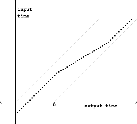 |
Figure 7.17 shows the relationship
between input and output time in a variable delay line. The delay
line is assumed to have a fixed maximum length ![]() .
At each sample of output (corresponding to a point on the
horizontal axis), we output one (possibly interpolated) sample of
the delay line's input. The vertical axis shows which sample
(integer or fractional) to use from the input signal. Letting
.
At each sample of output (corresponding to a point on the
horizontal axis), we output one (possibly interpolated) sample of
the delay line's input. The vertical axis shows which sample
(integer or fractional) to use from the input signal. Letting
![]() denote the output sample number, the
vertical axis shows the quantity
denote the output sample number, the
vertical axis shows the quantity ![]() , where
, where
![]() is the (time-varying) delay in samples.
If we denote the input sample location by:
is the (time-varying) delay in samples.
If we denote the input sample location by:
There remains one difference between delay lines and wavetables:
the material in the delay line is constantly being refreshed. Not
only can we not read into the future, but, if the the delay line is
![]() samples in length, we can't read further
than
samples in length, we can't read further
than ![]() samples into the past either:
samples into the past either:
Returning to Section 2.2, the Momentary Transposition
Formulas for Wavetables predict that the sound emerging from the
delay line will be transposed by a factor ![]() given
by:
given
by:
This is called the Doppler effect, and it occurs in nature as well. The air that sound travels through can sometimes be thought of as a delay line. Changing the length of the delay line corresponds to moving the listener toward or away from a stationary sound source; the Doppler effect from the changing path length works precisely the same in the delay line as it would be in the physical air.
Returning to Figure 7.17, we can predict that there is no pitch shift at the beginning, but then when the slope of the path decreases the pitch will drop for an interval of time before going back to the original pitch (when the slope returns to one). The delay time can be manipulated to give any desired transposition, but the greater the transposition, the less long we can maintain it before we run off the bottom or the top of the diagonal region.