Most signals aren't periodic, and even a periodic one might have
an unknown period. So we should be prepared to do Fourier analysis
on signals without the comforting assumption that the signal to
analyze repeats at a fixed period ![]() . Of course, we
can simply take
. Of course, we
can simply take ![]() samples of the signal and make
it periodic; this is essentially what we did in the previous
section, in which a pure sinusoid gave us the complicated Fourier
transform of Figure 9.3, part
(b).
samples of the signal and make
it periodic; this is essentially what we did in the previous
section, in which a pure sinusoid gave us the complicated Fourier
transform of Figure 9.3, part
(b).
However, it would be better to get a result in which the
response to a pure sinusoid were better localized around the
corresponding value of ![]() . We can accomplish this using
the enveloping technique shown in Figure 2.7 (page
. We can accomplish this using
the enveloping technique shown in Figure 2.7 (page ![]() ).
Applying this technique to Fourier analysis will not only improve
our analyses, but will also shed new light on the enveloping
looping sampler of Chapter 2.
).
Applying this technique to Fourier analysis will not only improve
our analyses, but will also shed new light on the enveloping
looping sampler of Chapter 2.
Given a signal x[n], periodic or not, defined on the points from
![]() to
to ![]() , the technique is
to envelope the signal before doing the Fourier analysis. The
envelope shape is known as a window function. Given a window function
, the technique is
to envelope the signal before doing the Fourier analysis. The
envelope shape is known as a window function. Given a window function
![]() , the windowed Fourier transform is:
, the windowed Fourier transform is:
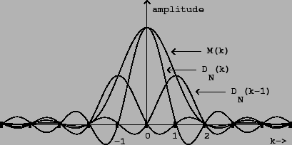 |
The main lobe of ![]() is four harmonics wide,
twice the width of the main lobe of the Dirichlet kernel. The
sidelobes, on the other hand, have much smaller magnitude. Each
sidelobe of
is four harmonics wide,
twice the width of the main lobe of the Dirichlet kernel. The
sidelobes, on the other hand, have much smaller magnitude. Each
sidelobe of ![]() is a sum of three sidelobes of
is a sum of three sidelobes of
![]() , one attenuated by
, one attenuated by ![]() and the others, opposite in sign, attenuated by
and the others, opposite in sign, attenuated by ![]() . They do not cancel out perfectly but they do cancel out
fairly well.
. They do not cancel out perfectly but they do cancel out
fairly well.
The sidelobes reach their maximum amplitudes near their
midpoints, and we can estimate their amplitudes there, using the
approximation:
This implies that applying a Hann window will allow us to isolate sinusoidal components from each other better in a Fourier transform (than if no Hann window is applied.) If a signal has many sinusoidal components, the sidelobes engendered by each one will interfere with the main lobe of all the others. Reducing the amplitude of the sidelobes reduces this interference.
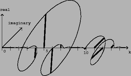 |
Figure 9.6 shows a Hann-windowed Fourier
analysis of a signal with two sinusoidal components. The two are
separated by about 5 times the fundamental frequency ![]() , and for each we see clearly the shape of the Hann
window's Fourier transform. Four points of the Fourier analysis lie
within the main lobe of
, and for each we see clearly the shape of the Hann
window's Fourier transform. Four points of the Fourier analysis lie
within the main lobe of ![]() corresponding to each
sinusoid. The amplitude and phase of the individual sinusoids are
reflected in those of the (four-point-wide) peaks. The four points
within a peak which happen to fall at integer values
corresponding to each
sinusoid. The amplitude and phase of the individual sinusoids are
reflected in those of the (four-point-wide) peaks. The four points
within a peak which happen to fall at integer values ![]() are successively one half cycle out of phase.
are successively one half cycle out of phase.
To fully resolve the partials of a signal, we should choose an
analysis size ![]() large enough so that
large enough so that ![]() is no more than a quarter of the frequency
separation between neighboring partials. For a periodic signal, for
example, the partials are separated by the fundamental frequency.
For the analysis to fully resolve the partials, the analysis period
is no more than a quarter of the frequency
separation between neighboring partials. For a periodic signal, for
example, the partials are separated by the fundamental frequency.
For the analysis to fully resolve the partials, the analysis period
![]() must be at least four periods of the
signal.
must be at least four periods of the
signal.
In some applications it works to allow the peaks to overlap as long as the center of each peak is isolated from all the other peaks; in this case the four-period rule may be relaxed to three or even slightly less.