Suppose you wish to fade a signal in over a period of ten
seconds--that is, you wish to multiply it by an
amplitude-controlling signal ![]() which rises from 0
to 1 in value over
which rises from 0
to 1 in value over ![]() samples, where
samples, where ![]() is the sample rate. The most obvious choice would be a
linear ramp:
is the sample rate. The most obvious choice would be a
linear ramp:
![]() . But this will not turn out to
yield a smooth increase in perceived loudness. Over the first
second
. But this will not turn out to
yield a smooth increase in perceived loudness. Over the first
second ![]() rises from
rises from ![]() dB to
-20 dB, over the next four by another 14 dB, and over the remaining
five, only by the remaining 6 dB. Over most of the ten second
period the rise in amplitude will be barely perceptible.
dB to
-20 dB, over the next four by another 14 dB, and over the remaining
five, only by the remaining 6 dB. Over most of the ten second
period the rise in amplitude will be barely perceptible.
Another possibility would be to ramp ![]() exponentially, so that it rises at a constant rate in dB. You would
have to fix the initial amplitude to be inaudible, say 0 dB (if we
fix unity at 100 dB). Now we have the opposite problem: for the
first five seconds the amplitude control will rise from 0 dB
(inaudible) to 50 dB (pianissimo); this part of the fade-in should
only have taken up the first second or so.
exponentially, so that it rises at a constant rate in dB. You would
have to fix the initial amplitude to be inaudible, say 0 dB (if we
fix unity at 100 dB). Now we have the opposite problem: for the
first five seconds the amplitude control will rise from 0 dB
(inaudible) to 50 dB (pianissimo); this part of the fade-in should
only have taken up the first second or so.
A more natural progression would perhaps have been to regard the fade-in as a timed succession of dynamics, 0-ppp-pp-p-mp-mf-f-ff-fff, with each step taking roughly one second.
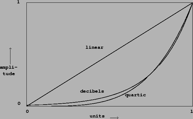
A fade-in ideally should obey some scale in between logarithmic
and linear. A somewhat arbitrary choice, but useful in practice, is
the quartic curve:
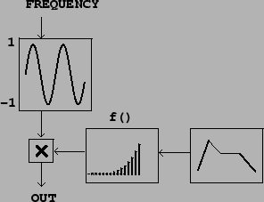
Figure 4.3 shows three amplitude
transfer functions:
 |
We can think of the three curves as showing transfer functions,
from an abstract control (ranging from 0 to 1) to a linear
amplitude. After we choose a suitable transfer function ![]() , we can compute a corresponding amplitude control signal; if
we wish to ramp over
, we can compute a corresponding amplitude control signal; if
we wish to ramp over ![]() samples from silence to unity
gain, the control signal would be:
samples from silence to unity
gain, the control signal would be: