


Next: Time-varying coefficients Up: Designing
filters Previous: Stretching the unit circle
Contents Index
We can apply the transformation  to
convert the Butterworth filter into a high-quality band-pass filter
with center frequency
to
convert the Butterworth filter into a high-quality band-pass filter
with center frequency  . A further transformation
can then be applied to shift the center frequency to any desired
value
. A further transformation
can then be applied to shift the center frequency to any desired
value  between 0 and
  . The
transformation will be of the form,
. The
transformation will be of the form,
where  and
and  are real numbers and
not both are zero. This is a particular case of the general form
given above for unit-circle-preserving rational functions. We have
are real numbers and
not both are zero. This is a particular case of the general form
given above for unit-circle-preserving rational functions. We have
 and
and  , and
the top and bottom halves of the unit circle are transformed
symmetrically (if
, and
the top and bottom halves of the unit circle are transformed
symmetrically (if  goes to
  then
then  goes to
  ). The qualitative effect of the transformation
 is to squash points of the unit circle
toward
is to squash points of the unit circle
toward  or
or  .
.
In particular, given a desired center frequency , we wish to choose so that:
If we leave  as before, and let
 be the transfer function for a low-pass
Butterworth filter, then the combined filter with transfer function
be the transfer function for a low-pass
Butterworth filter, then the combined filter with transfer function
 will be a band-pass filter with
center frequency . Solving for and
gives:
will be a band-pass filter with
center frequency . Solving for and
gives:
The new transfer function, , will have
 poles and zeros (if
 is the degree of the Butterworth filter
).
is the degree of the Butterworth filter
).
Knowing the transfer function is good, but even better is
knowing the locations of all the poles and zeros of the new filter,
which we need to be able to compute it using elementary filters. If
is a pole of the transfer function
 , that is, if
  , then
  must be a pole of
. The same goes for zeros. To find a pole or
zero of
must be a pole of
. The same goes for zeros. To find a pole or
zero of  we set
  , where
is a pole or zero of , and
solve for . This gives:
, where
is a pole or zero of , and
solve for . This gives:
(Here and are as given above
and we have used the fact that  ). A
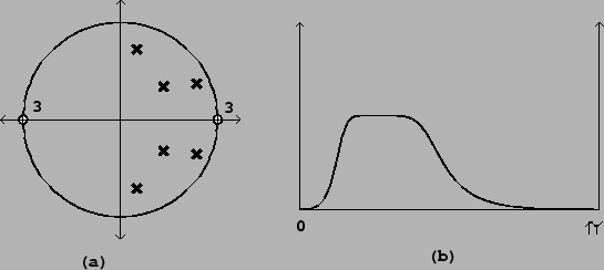
sample pole-zero plot and frequency response of
are shown in Figure 8.20.
). A
sample pole-zero plot and frequency response of
are shown in Figure 8.20.
Figure 8.20: Butterworth
band-pass filter: (a) pole-zero diagram; (b) frequency response.
The center frequency is  . The bandwidth depends
both on center frequency and on the bandwidth of the original
Butterworth low-pass filter used.
. The bandwidth depends
both on center frequency and on the bandwidth of the original
Butterworth low-pass filter used.
 |
Next: Time-varying coefficients Up: Designing
filters Previous: Stretching the unit circle
Contents Index
Miller Puckette 2006-12-30