Sampling

``Sampling" is nothing more than recording a live signal into a wavetable, and then later playing it out again. (In commercial samplers the entire wavetable is usually called a ``sample" but to avoid confusion we'll only use the word ``sample" here to mean a single number in an audio signal.)

At its simplest, a sampler is simply a wavetable oscillator, as was shown in Figure 2.3. However, in the earlier discussion we imagined playing the oscillator back at a frequency high enough to be perceived as a pitch, at least 30 Hertz or so. In the case of sampling, the frequency is usually lower than 30 Hertz, and so the period, at least 1/30 second and perhaps much more, is long enough that you can hear the individual cycles as separate events.

Going back to Figure 2.2, suppose that instead of 40 points the wavetable $x[n]$ is a one-second recording, at an original sample rate of 44100, so that it has 44100 points; and let $y[n]$ in part (b) of the figure have a period of 22050 samples. This corresponds to a frequency of 2 Hertz. But what we hear is not a pitched sound at 2 cycles per second (that's too slow to hear as a pitch) but rather, we hear the original recording $x[n]$ played back repeatedly at double speed. We've just reinvented the sampler.

In general, if we assume the sample rate $R$ of the recording is the same as the output sample rate, if the wavetable has $N$ samples, and if we index it with a sawtooth wave of period $M$, the sample is sped up or slowed down by a factor of $N/M$, equal to $N f / R$ if $f$ is the frequency in Hertz of the sawtooth. If we denote the transposition factor by $t$ (so that, for instance, $t=3/2$ means transposing upward a perfect fifth), and if we denote the transposition in half-steps by $h$, then we get the Transposition Formulas for Looping Wavetables:

$$t = {N / M} = {{N f} / R}$$

$$h = 12 \, {\log _ 2} \left ( {N \over M} \right ) = 12 \, {\log _ 2} \left ( {N f \over R} \right )$$

Frequently the desired transposition in half-steps ($h$) is known and the formula must be solved for either $f$ or $N$:

$$f = {{2^{h/12} R} \over N}$$

$$N = {{2^{h/12} R} \over f}$$

So far we have used a sawtooth as the input wave $y[t]$, but, as suggested in parts (d) and (e) of Figure 2.2, we could use anything we like as an input signal. In general, the transposition may be time dependent and is controlled by the rate of change of the input signal.

The transposition multiple $t$ and the transposition in half-steps $h$ are then given by the Momentary Transposition Formulas for Wavetables:

$$t[n] = \left \vert y[n] - y[n-1] \right \vert$$

$$h[n] = 12 {{\log_2} \left \vert y[n] - y[n-1] \right \vert}$$

(Here the enclosing bars ``$\vert$" mean absolute value.) For example, if $y[n] = n$, then $z[n] = x[n]$ so we hear the wavetable at its original pitch, and this is what the formula predicts since, in that case,

$$y[n]-y[n-1] = 1$$

On the other hand, if $y[n] = 2n$, then the wavetable is transposed up an octave, consistent with

$$y[n]-y[n-1] = 2$$

If values of $y[n]$ are decreasing with $n$, you hear the sample backward, but the transposition formula still gives a positive multiplier. This all agrees with the earlier Transposition Formula for Looping Wavetables; if a sawtooth ranges from $0$ to $N$, $f$ times per second, the difference of successive samples is just $N f / R$--except at the sample at the beginning of each new cycle.

It's well known that transposing a recording also transposes its timbre--this is the ``chipmunk" effect. Not only are any periodicities (such as might give rise to pitch) transposed, but so are the frequencies of the overtones. Some timbres, notably those of vocal sounds, have characteristic frequency ranges in which overtones are stronger than other nearby ones. Such frequency ranges are also transposed, and this is is heard as a timbre change. In language that will be made more precise in Section 5.1, we say that the spectral envelope is transposed along with the pitch or pitches.

In both this and the preceding section, we have considered playing wavetables periodically. In Section 2.1 the playback repeated quickly enough that the repetition gives rise to a pitch, say between 30 and 4000 times per second, roughly the range of a piano. In the current section we assumed a wavetable one second long, and in this case ``reasonable" transposition factors (less than four octaves up) would give rise to a rate of repetition below 30, usually much lower, and going down as low as we wish.

The number 30 is significant for another reason: it is roughly the maximum number of separate events the ear can discern per second; for instance, 30 vocal phonemes, or melodic notes, or attacks of a snare drum are about the most we can hope to crowd into a second before our ability to distinguish them breaks down.

A continuum exists between samplers and wavetable oscillators, in that the patch of Figure 2.3 can either be regarded as a sampler (if the frequency of repetition is less than about 20 Hertz) or as a wavetable oscillator (if the frequency is greater than about 40 Hertz). It is possible to move continuously between the two regimes. Furthermore, it is not necessary to play an entire wavetable in a loop; with a bit more arithmetic we can choose sub-segments of the wavetable, and these can change in length and location continuously as the wavetable is played.

The practice of playing many small segments of a wavetable in rapid succession is often called granular synthesis. For much more discussion of the possibilities, see [Roa01].

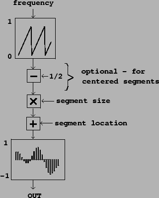
Figure 2.5 shows how to build a very simple looping sampler. In the figure, if the frequency is $f$ and the segment size in samples is $s$, the output transposition factor is given by $t = fs/R$, where R is the sample rate at which the wavetable was recorded (which need not equal the sample rate the block diagram is working at.) In practice, this equation must usually be solved for either $f$ or $s$ to attain a desired transposition.

In the figure, a sawtooth oscillator controls the location of wavetable lookup, but the lower and upper values of the sawtooth aren't statically specified as they were in Figure 2.3; rather, the sawtooth oscillator simply ranges from 0 to 1 in value and the range is adjusted to select a desired segment of samples in the wavetable.

It might be desirable to specify the segment's location $l$ either as its left-hand edge (its lower bound) or else as the segment's midpoint; in either case we specify the length $s$ as a separate parameter. In the first case, we start by multiplying the sawtooth by $s$, so that it then ranges from $0$ to $s$; then we add $l$ so that it now ranges from $l$ to $l+s$. In order to specify the location as the segment's midpoint, we first subtract $1/2$ from the sawtooth (so that it ranges from $-1/2$ to $1/2$), and then as before multiply by $s$ (so that it now ranges from $-s/2$ to $s/2$) and add $l$ to give a range from $l-s/2$ to $l+s/2$.

Figure 2.5: A simple looping sampler, as yet with no amplitude control. There are inputs to control the frequency and the segment size and location. The ``-" operation is included if we wish the segment location to be specified as the segment's midpoint; otherwise we specify the location of the left end of the segment.

In the looping sampler, we will need to worry about maintaining continuity between the beginning and the end of segments of the wavetable; we'll take this up in the next section.

A further detail is that, if the segment size and location are changing with time (they might be digital audio signals themselves, for instance), they will affect the transposition factor, and the pitch or timbre of the output signal might waver up and down as a result. The simplest way to avoid this problem is to synchronize changes in the values of $s$ and $l$ with the regular discontinuities of the sawtooth; since the signal jumps discontinuously there, the transposition is not really defined there anyway, and, if you are enveloping to hide the discontinuity, the effects of changes in $s$ and $l$ are hidden as well.