In the previous chapter we treated audio signals as if they always flowed by in a continuous stream at some sample rate. The sample rate isn't really a quality of the audio signal, but rather it specifies how fast the individual samples should flow into or out of the computer. But the audio signal is at bottom just a sequence of numbers, and in practice we don't have to assume that they will be ``played" linearly at all. Another, complementary view is that they can be stored in memory, and, later, they can be read back in any order--forward, backward, back and forth, or totally at random. A huge range of new possibilities opens up, one that will never be exhausted.
For many years (roughly 1950-1990), magnetic tape served as the main storage medium for sounds. Tapes were passed back and forth across magnetic pickups to render them in real time. Since 1995 or so, the predominant method of sound storage has been to keep them as digital audio signals, which are read back with much greater freedom and facility than were the magnetic tapes. Many modes of use dating from the tape era are still current, including cutting, duplication, speed change, and time reversal. Other techniques, such as waveshaping, have come into their own only in the digital era.
Suppose we have a stored digital audio signal, which is just a
sequence of numbers ![]() for
for
![]() , where
, where ![]() is
the size in samples of the stored signal. Then if we have an input
signal
is
the size in samples of the stored signal. Then if we have an input
signal ![]() (which we assume to be flowing in real
time), we can use its values as indices to look up values of the
stored signal
(which we assume to be flowing in real
time), we can use its values as indices to look up values of the
stored signal ![]() . This operation, called wavetable lookup, gives us a new
signal,
. This operation, called wavetable lookup, gives us a new
signal, ![]() , calculated as:
, calculated as:
 |
Two complications arise. First, the input values, ![]() , might lie outside the range
, might lie outside the range ![]() , in
which case the wavetable
, in
which case the wavetable ![]() has no value and the
expression for the output
has no value and the
expression for the output ![]() is undefined. In
this situation we might choose to anything negative and
is undefined. In
this situation we might choose to anything negative and ![]() for anything N or
greater. Alternatively, we might prefer to wrap them around end to
end. Here we'll adopt the convention that out-of-range samples are
always clipped; when we need wraparound, we'll introduce another
signal processing block to do it for us.
for anything N or
greater. Alternatively, we might prefer to wrap them around end to
end. Here we'll adopt the convention that out-of-range samples are
always clipped; when we need wraparound, we'll introduce another
signal processing block to do it for us.
The second complication is that the input values need not be
integers; in other words they might fall between the points of the
wavetable. In general, this is addressed by choosing some scheme
for interpolating between the points of the wavetable. For the
moment, though, we'll just round down to the nearest integer below
the input. This is called noninterpolating wavetable lookup, and its full
definition is:
![\begin{displaymath} z[n] = \left \{ { \begin{array}{ll} x[ \lfloor y[n] \rflo... ...x[N-1] & \mbox{if $y[n] \ge N-1$} \ \end{array} } \right . \end{displaymath}](img123.png)
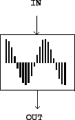
Pictorally, we use ![]() (a number) as a location
on the horizontal axis of the wavetable shown in figure 2.1, and the output,
(a number) as a location
on the horizontal axis of the wavetable shown in figure 2.1, and the output, ![]() , is whatever we get on the vertical axis; and the same
for
, is whatever we get on the vertical axis; and the same
for ![]() and
and ![]() and so on. The
``natural" range for the input
and so on. The
``natural" range for the input ![]() is
is
![]() . This is different from the
usual range of an audio signal suitable for output from the
computer, which ranges from -1 to 1 in our units. We'll see later
that the range of input values, nominally from 0 to
. This is different from the
usual range of an audio signal suitable for output from the
computer, which ranges from -1 to 1 in our units. We'll see later
that the range of input values, nominally from 0 to ![]() ,
contracts slightly if interpolating lookup is used.
,
contracts slightly if interpolating lookup is used.
Figure 2.2 shows a wavetable
(a) and the result of using two different input signals as lookup
indices into it. The wavetable contains 40 points, which are
numbered from 0 to 39. In part (b) of the figure, a sawtooth wave is used as the input signal
![]() . A sawtooth wave is nothing but a ramp
function repeated end to end. In this case the sawtooth's range is
from
. A sawtooth wave is nothing but a ramp
function repeated end to end. In this case the sawtooth's range is
from ![]() to
to ![]() (this is shown in
the vertical axis). The sawtooth wave thus scans the wavetable from
left to right--from the beginning point 0 to the endpoint 39--and
does so every time it repeats. Over the fifty points shown in
Figure 2.2(b) the sawtooth wave
makes two and a half cycles. Its period is twenty samples, or in
other words the frequency in Hertz is
(this is shown in
the vertical axis). The sawtooth wave thus scans the wavetable from
left to right--from the beginning point 0 to the endpoint 39--and
does so every time it repeats. Over the fifty points shown in
Figure 2.2(b) the sawtooth wave
makes two and a half cycles. Its period is twenty samples, or in
other words the frequency in Hertz is ![]() .
.
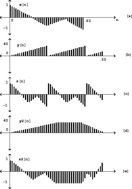 |
Part (c) of figure 2.2 shows
the result of applying wavetable lookup, using the table
![]() , to the signal
, to the signal ![]() . Since
the sawtooth input simply reads out the contents of the wavetable
from left to right, repeatedly, at a constant rate of precession,
the result will be a new periodic signal, whose waveform (shape) is
derived from
. Since
the sawtooth input simply reads out the contents of the wavetable
from left to right, repeatedly, at a constant rate of precession,
the result will be a new periodic signal, whose waveform (shape) is
derived from ![]() and whose frequency is determined by
the sawtooth wave
and whose frequency is determined by
the sawtooth wave ![]() .
.
Parts (d) and (e) of figure 2.2 show an example of reading the
wavetable in a nonuniform way; since the inputs signal rises from
![]() to
to ![]() and then later
recedes to
and then later
recedes to ![]() , we see the wavetable appear first
forward, then frozen at its endpoint, then backward. The table is
scanned from left to right and then, more quickly, from right to
left. As in the previous example the incoming signal controls the
speed of precession while the output's amplitude is that of the
wavetable.
, we see the wavetable appear first
forward, then frozen at its endpoint, then backward. The table is
scanned from left to right and then, more quickly, from right to
left. As in the previous example the incoming signal controls the
speed of precession while the output's amplitude is that of the
wavetable.