Linear and Curved Amplitude Shapes

Suppose you wish to fade a signal in over a period of ten seconds--that is, you wish to multiply it by an amplitude-controlling signal $y[n]$ which rises from 0 to 1 in value over $10R$ samples, where $R$ is the sample rate. The most obvious choice would be a linear ramp: $y[n] = n/(10R)$. But this will not turn out to yield a smooth increase in perceived loudness. Over the first second $y[n]$ rises from $-\infty$ dB to -20 dB, over the next four by another 14 dB, and over the remaining five, only by the remaining 6 dB. Over most of the ten second period the rise in amplitude will be barely perceptible.

Another possibility would be to ramp $y[n]$ exponentially, so that it rises at a constant rate in dB. You would have to fix the initial amplitude to be inaudible, say 0 dB (if we fix unity at 100 dB). Now we have the opposite problem: for the first five seconds the amplitude control will rise from 0 dB (inaudible) to 50 dB (pianissimo); this amount of rise should have only taken up the first second or so.

The natural progression should perhaps have been: 0-ppp-pp-p-mp-mf-f-ff-fff, so that each increase of one dynamic marking would take roughly one second, and would correspond to one "step" in loudness.

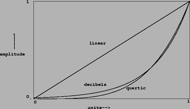
We appear to need some scale in between logarithmic and linear. A somewhat arbitrary choice, but useful in practice, is the quartic curve:

$$y[n] = {{ \left ( {{n} \over {N}} \right ) } ^ 4} ,$$

where $N$ is the number of samples to fade in over (in the example above, it's $10R$). So, over the second (of the ten) we would rise to -80 dB, after five seconds to -24 dB, and after nine, about -4 dB.

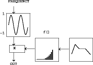
Figure 4.3 shows three amplitude transfer functions:

$${f_1} (x) = x \hspace{0.2in} \mathrm{(linear),}$$

$$\ \ \ \ \ \ \ %% {f_2} (x) = 10^{2x} \hspace{0.2in}\mathrm{(dB\ to\ linear),}$$

$${f_3} (x) = {x^4} \hspace{0.2in}\mathrm{(quartic).}$$

The second function converts from dB to linear, arranged so that the input range, from 0 to 1, corresponds to 40 dB. (This input range of 40 dB corresponds to a reasonable dynamic range, allowing 5 dB for each of 8 steps in dynamic.) The quartic curve imitates the exponential (dB) curve fairly well for higher amplitudes, but drops off more rapidly for small amplitudes, reaching true zero at right (whereas the exponential curve only goes down to $1/100$.)

Figure 4.3: Three amplitude transfer functions. The horizontal axis is in linear, logarithmic, or fourth-root units depending on the curve.

We can think of the three curves as showing transfer functions, from an abstract control (ranging from 0 to 1) to a linear amplitude. After we choose a suitable transfer function $f$, we can compute a corresponding amplitude control signal; if we wish to ramp over $N$ samples from silence to unity gain, the control signal would be:

$$y[n] = f(n/N) .$$

A block diagram for this is shown in Figure 4.4. Here we are introducing a new type of block to represent the application of a transfer function. For now we won't worry about its implementation; depending on the function desired, this might be best done arithmetically or using table lookup.

Figure 4.4: Using a transfer function to alter the shape of amplitude curves.