Pulse trains

In the wavetable formulation, the pulse train can be made by a stretched wavetable:

$${M_a}(\phi) = W (a \phi),$$

where $-\pi \le \phi \le \pi$ is the phase. The function $W$ should be zero at and beyond the points $-\pi$ and $\pi$, and rise to a maximum at 0. A possible choice for the function $W$ is

$$W(\phi) = {1\over2} \left ( \cos(\phi) + 1 \right )$$

which is graphed in part (a) of Figure 6.4. This is known as the Hanning window function; it will come up again in chapter .

Figure: Pulse width modulation using the Hanning window function: a. the function $W(\phi)=(1+\cos(\phi))/2$; b. the function repeated at a duty cycle of 100% (modulation index $a=1$); c. the function at a 50% duty cycle ($a=2$).

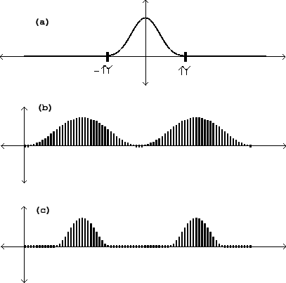
Realizing this as a repeating waveform, we get a succession of (appropriately sampled) copies of the function $W$, whose duty cycle is $1/a$ (parts b and c of the figure). If you don't wish the copies to overlap we require $a$ to be at least 1. If you want overlap the best strategy is to duplicate the block diagram (Figure 6.3) out of phase, as described in Section 2.4 and realized in Section 2.6.5.

In the ring modulated waveshaping formulation, the shape of the formant is determined by a modulation term

$$m[n] = f (a \cos(\omega_m n))$$

For small values of the index $a$, the modulation term varies only slightly from the constant value $f(0)$, so most of the energy is concentrated at DC. As $a$ increases, the energy spreads out among progressively higher harmonics of the fundamental $\omega_m$. Depending on the function $f$, this spread may be orderly or disorderly. An orderly spread may be desirable and then again may not, depending on whether our goal is a predictable spectrum or a wide range of different (and perhaps hard-to-predict) spectra.

A waveshaping function that gives well-behaved, simple and predictable results was already developed in section 5.5.5. Using the function

$$f(x) = {e ^ x}$$

and normalizing suitably, we get the spectra shown in figure 5.13. A slight rewriting of the waveshaping modulator for this choice of $f$ (and taking the renormalization into account) gives:

$${m_a}(\omega n) = {e^{a \cdot (\cos(\omega n) - 1))}}$$

$$= e ^ { { -\left [ b \sin {\omega \over 2} \right ] } ^2 }$$

where ${b^2}=2a$ so that $b$ is proportional to the bandwidth. This can be rewritten as

$${m_a}(\omega n) = g ( b \sin {\omega \over 2} n )$$

$$g(x) = e ^ {- x ^ 2}$$

Except for a missing normalization factor, this is a Gaussian distribution, sometimes called a ``bell curve". The amplitudes of the harmonics are given by Bessel ``I" type functions.

Another good choice is the (again unnormalized) Cauchy distribution:

$$h(x) = {1\over{1 + {x^2}}}$$

which gives rise to a spectrum of exponentially falling harmonics:

$$h(b \sin(\omega n / 2)) = G \cdot \left ( {1\over 2} + H \cos(\omega n) + {H^2} \cos(2 \omega n) + \cdots \right )$$

where $G$ and $H$ are functions of the index $b$ (exact formulas are given in []).

In both this and the Gaussian case above, the bandwidth (counted in peaks, i.e., units of $\omega$) is roughly proportional to the index $b$, and the amplitude of the DC term (the peak of the spectrum) is roughly proportional to $1/(1+b)$ . For either waveshaping function ($g$ or $c$), if $b$ is larger than about 2, the waveshape of ${m_a}(\omega n)$ is approximately a (forward or backward) scan of the transfer function, and so this and the earlier example (the ``wavetable formulation") both look like pulses whose widths decrease as the specified bandwidth increases.

Before considering more complicated carrier signals to go with the modulators we've seen so far, it is instructive to see what multiplication by a pure sinusoid gives us as waveforms and spectra. Figure 6.5 shows the result of multiplying two different pulse trains by a sinusoid at the sixth partial:

$$cos(6 \omega n) {M_a}(\omega n)$$

where the index of modulation $a$ is two in both cases. In part (a) $M_a$ is the stretched Hanning windowing function; part (b) shows waveshaping via the unnormalized Cauchy distribution. One period of each waveform is shown.

Figure 6.5: Audio signals resulting from multiplying a cosine (partial number 6) by pulse trains: (a). windowing function from the wavetable formulation; (b) waveshaping output using the Gaussian lookup function.

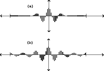In both cases we see, in effect, the sixth harmonic (the carrier signal) enveloped into a wave packet centered at the middle of the cycle, where the phase of the sinusoid is zero. Changing the frequency of the sinusoid changes the center frequency of the formant; changing the width of the packet (the proportion of the waveform during which the sinusoid is strong) changes the bandwidth. Note that the stretched Hanning window function is zero at the beginning and end of the period, unlike the waveshaping packet.

Figure 6.6 shows how the specific shape of the formant depends on the method of production. The stretched wavetable form (part (a) of the figure) behaves well in the neighborhood of the peak, but somewhat oddly starting at four partials' distance from the peak, past which we see what are called sidelobes: spurious extra peaks at lower amplitude than the central peak. As the analysis of Section 2.4 predicts, the entire formant, sidelobes and all, stretches or contracts inversely as the pulse train is contracted or stretched in time.

Figure 6.6: Spectra of three ring-modulated pulse trains: (a). the Hanning window function, 50% duty cycle (corresponding to an index of 2); (b), a waveshaping pulse train using a Gaussian transfer function; (c) the same, with a Cauchy transfer function. Amplitudes are in decibels.

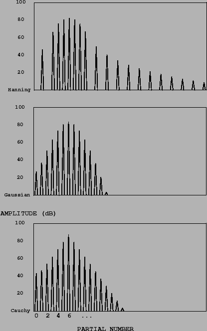The first, strongest sidelobes on either side are about 37 dB lower in amplitude than the main peak. Further sidelobes drop off slowly when expressed in decibels; the amplitudes decrease as the square of the distance from the center peak so that the sixth sidelobe to the right, three times further than the first one from the center frequency, is about twenty decibels further down. The effect of these sidelobes is often audible as a slight buzziness in the sound.

This formant shape may be made arbitrarily fat (i.e., high bandwidth), but there is a limit on how thin it can be made, since the duty cycle of the waveform cannot exceed 100%. At this maximum duty cycle the formant strength drops to zero at two harmonics' distance from the center peak. If a still lower bandwidth is needed, waveforms may be made to overlap as described in section 2.6.5.

Parts (b) and (c) of the figure show formants generated using ring modulated waveshaping, with Gaussian and Cauchy transfer functions. The index of modulation is two in both cases (the same as for the Hanning window of part (a)), and the bandwidth is comparable to that of the Hanning example. In these examples there are no sidelobes, and moreover, the index of modulation may be dropped all the way to zero, giving a pure sinusoid; there is no lower limit on bandwidth. On the other hand, since the waveform does not reach zero at the ends of a cycle, this type of pulse train cannot be used to window an arbitrary wavetable, as the Hanning pulse train could.

The Cauchy example is particularly easy to build designer spectra from, since the shape of the formant is a perfect Isosocles triangle, when graphed in decibels. On the other hand, the Gaussian example gathers more energy to the neighborhood of the formant, and drops off faster at the tails, and so has a cleaner sound.