A favorite use of variable delay lines is to alter the pitch of an incoming sound using the Doppler effect. It may be desirable to alter the pitch variably (randomly or periodically, for example), or else to maintain a fixed musical interval of transposition over a length of time.
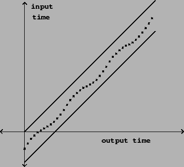
Returning to Figure 7.17, we see that with a single variable delay line we can maintain any desired pitch shift for a limited interval of time, but if we wish to sustain a fixed transposition we will always eventually land outside the diagonal strip of admissible delay times. In the simplest scenario, we simply vary the transposition up and down so as to remain in the strip.
 |
This works, for example, if we wish to apply vibrato to a sound
as shown in Figure 7.19. Here the delay
function is
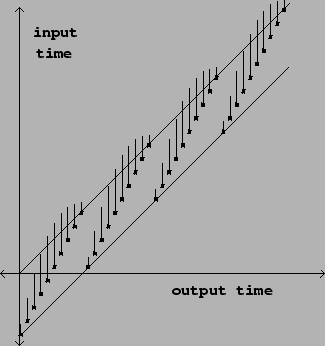 |
Suppose, on the other hand, that we wish to maintain a constant transposition over a longer interval of time. In this case we can't maintain the transposition forever, but it is still possible to maintain it over fixed intervals of time broken by discontinuous changes, as shown in Figure 7.20. The delay time is the output of a suitably normalized sawtooth function, and the output of the variable delay line is enveloped as shown in the figure to avoid discontinuities.
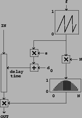 |
This is accomplished as shown in Figure 7.21. The output of the sawtooth generator is used
in two ways. First it is adjusted to run between the bounds
![]() and
and ![]() , and this
adjusted sawtooth controls the delay time, in samples. The initial
delay
, and this
adjusted sawtooth controls the delay time, in samples. The initial
delay ![]() should be at least enough to make the
variable delay feasible; for four-point interpolation it must be at
least one sample. Larger values of
should be at least enough to make the
variable delay feasible; for four-point interpolation it must be at
least one sample. Larger values of ![]() add a
constant, additional delay to the output; this is usually offered
as a control in a pitch shifter since it is essentially free. The
quantity
add a
constant, additional delay to the output; this is usually offered
as a control in a pitch shifter since it is essentially free. The
quantity ![]() is sometimes called the window size. It corresponds roughly to the sample
length in a looping sampler (Section 2.2).
is sometimes called the window size. It corresponds roughly to the sample
length in a looping sampler (Section 2.2).
The sawtooth output is also used to envelope the output in
exactly the same way as in the enveloped wavetable sampler of
Figure 2.7 (Page ![]() ).
The envelope is zero at the points where the sawtooth wraps around,
and in between, rises smoothly to a maximum value of 1 (for unit
gain).
).
The envelope is zero at the points where the sawtooth wraps around,
and in between, rises smoothly to a maximum value of 1 (for unit
gain).
If the frequency of the sawtooth wave is ![]() (in
cycles per second), then its value sweeps from 0 to 1 every
(in
cycles per second), then its value sweeps from 0 to 1 every
![]() samples (where
samples (where ![]() is the
sample rate). The difference between successive values is thus
is the
sample rate). The difference between successive values is thus
![]() . If we let
. If we let ![]() denote the
output of the sawtooth oscillator, then
denote the
output of the sawtooth oscillator, then
 |
The pitch shifter can transpose either upward (using negative
sawtooth frequencies, as in the figure) or downward, using positive
ones. Pitch shift is usually controlled by changing ![]() with
with ![]() fixed. To get a desired transposition
interval
fixed. To get a desired transposition
interval ![]() , set
, set
Although the frequency may be changed at will, even
discontinuously, ![]() must be changed more carefully. A
possible solution is to mute the output while changing
must be changed more carefully. A
possible solution is to mute the output while changing ![]() discontinuously; alternatively,
discontinuously; alternatively, ![]() may be ramped
continuously but this causes hard-to-control Doppler shifts.
may be ramped
continuously but this causes hard-to-control Doppler shifts.
A good choice of envelope is one half cycle of a sinusoid. If we
assume on average that the two delay outputs are uncorrelated (Page
![]() ),
the signal power from the two delay lines, after enveloping, will
add to a constant (since the sum of squares of the two envelopes is
one).
),
the signal power from the two delay lines, after enveloping, will
add to a constant (since the sum of squares of the two envelopes is
one).
Many variations exist on this pitch shifting algorithm. One classic variant uses a single delay line, with no enveloping at all. In this situation it is necessary to choose the point at which the delay time jumps, and the point it jumps to, so that the output stays continuous. For example, one could find a point where the output signal passes through zero (a ``zero crossing") and jump discontinuously to another one. Using only one delay line has the advantage that the signal output sounds more ``present". A disadvantage is that, since the delay time is a function of input signal value, the output is no longer a linear function of the input, so non-periodic inputs can give rise to artifacts such as difference tones.