Timbre stretching

The wavetable oscillator of Section 2.1, which we extended in Section 2.2 to encompass grabbing waveforms from arbitrary wavetables such as recorded sounds, may additionally be extended in a complementary way, that we'll refer to as timbre stretching, for reasons we'll develop in this section. There are also many other possible ways to extend wavetable synthesis, using for instance frequency modulation and waveshaping, but we'll leave them to later chapters.

The central idea of timbre stretching is to reconsider the idea of the wavetable oscillator as a mechanism for playing a stored wavetable (or part of one) end to end. There is no reason the end of one cycle has to coincide with the beginning of another. Instead, we could ask for copies of the waveform to be spaced with alternating segments of silence; or, going in the opposite direction, the waveform copies could be spaced more closely together so that they overlap. The single parameter available in Section 2.1--the frequency--has been heretofore used to control two separate aspects of the output: the period at which we start new copies of the waveform, and also the length of each individual copy. The idea of timbre stretching is to control the two independently.

Figure 2.9 shows the result of playing a wavetable in three ways. In each case the output waveform has period 20; in other words, the output frequency is $R/20$ if $R$ is the output sample rate. In part (a) of the figure, each copy of the waveform is played over 20 samples, so that the wave form fits exactly into the cycle with no gaps and no overlap. In part (b), although the period is still 20, the waveform is compressed into the middle half of the period (10 samples); or in other words, the duty cycle--the relative amount of time the waveform fills the cycle--equals 50 percent. The remaining 50 percent of the time, the output is zero.

Figure 2.9: A waveform is played at a period of 20 samples: (a) at 100 percent duty cycle; (b) at 50 percent; (c) at 200 percent

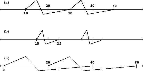In part (c), the waveform is stretched to 40 samples, and since it is still repeated every 20 samples, the waveforms overlap two to one. The duty cycle is thus 200 percent.

Suppose now that the 100 percent duty cycle waveform has a Fourier series (Section 1.7) equal to:

$${x_{100}}[n] = {a_0} + {a_1} \cos \left ( \omega n + {\phi... ...+ {a_2} \cos \left ( 2 \omega n + {\phi_2} \right ) + \cdots$$

where $\omega$ is the angular frequency (equal to $\pi/10$ in our example since the period is 20.) To simplify this example we won't worry about where the series must end, and will just let it go on forever.

We would like to relate this to the Fourier series of the other two waveforms in the example, in order to show how changing the duty cycle changes the timbre of the result. For the 50 percent duty cycle case (calling the signal ${x_{50}}[n]$), we observe that the waveform, if we replicate it out of phase by a half period and add the two, gives exactly the original waveform at twice the frequency:

$${x_{100}}[2n] = {x_{50}}[n] + {x_{50}}[n+{\pi \over \omega}]$$

where $\omega$ is the angular frequency (and so $\pi / \omega$ is half the period) of both signals. So if we denote the Fourier series of ${x_{50}}[n]$ as:

$${x_{50}}[n] = {b_0} + {b_1} \cos \left ( \omega n + {\thet... ... {b_2} \cos \left ( 2 \omega n + {\theta_2} \right ) + \cdots$$

and substitute the Fourier series for all three terms above, we get:

$${a_0} + {a_1} \cos \left ( 2 \omega n + {\phi_1} \right ) + {a_2} \cos \left ( 4 \omega n + {\phi_2} \right ) + \cdots$$

$$= {b_0} + {b_1} \cos \left ( \omega n + {\theta_1} \right... ... {b_2} \cos \left ( 2 \omega n + {\theta_2} \right ) + \cdots$$

$$+ {b_0} + {b_1} \cos \left ( \omega n + \pi + {\theta_1} ... ...\cos \left ( 2 \omega n + 2 \pi + {\theta_2} \right ) + \cdots$$

$$= 2 {b_0} + 2 {b_2} \cos \left ( 2 \omega n + {\theta_2} \... ... {b_4} \cos \left ( 4 \omega n + {\theta_4} \right ) + \cdots$$

and so

$${a_0} = 2{b_0}, \,\, {a_1} = 2{b_2}, \,\, {a_2} = 2{b_4}$$

and so on: the even partials of $x_{50}$, at least, are obtained by stretching the partials of $x_{100}$ out twice as far. (We don't yet know about the odd partials of $x_{50}$, and these might be in line with the even ones or not, depending on factors we can't control yet. Suffice it to say for the moment, that if the waveform connects smoothly with the horizontal axis at both ends, the odd partials will act globally like the even ones. To make this more exact we'll need Fourier analysis, which is developed in Chapter 9.)

Similarly, $x_{100}$ and $x_{200}$ are related in exactly the same way:

$${x_{200}}[2n] = {x_{100}}[n] + {x_{100}}[n+{\pi \over \omega}]$$

so that, if the amplitudes of the fourier series of $x_{200}$ are denoted by $c_0$, $c_1$, $\ldots$, we get:

$${c_0} = 2{a_0}, {c_1} = 2{a_2}, {c_2} = 2{a_4}, \ldots$$

so that the partials of $x_{200}$ are those of $x_{100}$ shrunk, by half, to the left.

We see that squeezing the waveform by a factor of 2 has the effect of stretching the Fourier series out by two, and on the other hand stretching the waveform by a factor of two squeezes the Fourier series by two. By the same sort of argument, in general it turns out that stretching the waveform by a factor of any positive number $f$ squeezes the overtones, in frequency, by the reciprocal $1/f$--at least approximately, and the approximation is at least fairly good if the waveform ``behaves well" at its ends. (As we'll see later, the waveform can always be forced to behave at least reasonably well by enveloping it as in Figure 2.7.)

Figure 2.10 shows the spectra of the three waveforms--or in other words the one waveform at three duty cycles--of Figure 2.9. The figure emphasizes the relationship between the three spectra by drawing curves through each, which, on inspection, turn out to be the same curve, only stretched differently; as the duty cycle goes up, the curve is both compressed to the left (the frequencies all drop) and amplified (stretched upward).

Figure 2.10: The Fourier series magnitudes for the waveforms shown in Figure 2.9. The horizontal axis is the harmonic number. We only ``hear" the coefficients for integer harmonic numbers; the continuous curves are the ``ideal" contours.

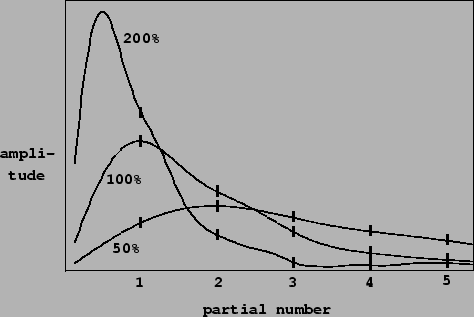The continuous curves have a very simple interpretation. Imagine squeezing the waveform into some tiny duty cycle, say 1 percent. The contour will be stretched by a factor of 100. Working backward, this would allow us to interpolate between each pair of consecutive points of the 100 percent duty cycle contour (the original one) with 99 new ones. Already in the figure the 50 percent duty cycle trace defines the curve with twice the resolution of the original one. In the limit, as the duty cycle gets arbitrarily small, the spectrum is filled in more and more densely; and the limit is the ``true" spectrum of the waveform.

This ``true" spectrum is only audible at suitably low duty cycles, though. The 200 percent duty cycle example actually misses the peak in the ideal (continuous) spectrum because the peak falls below the first harmonic. In general, higher duty cycles sample the ideal curve at lower resolutions.

Timbre stretching is an extremely powerful technique for generating sounds with systematically variable spectra. Combined with the possibilities of mixtures of waveforms (Section 2.1) and of snatching endlessly variable waveforms from recorded samples (Section 2.2), it is possible to generate all sorts of sounds. For example, the block diagram of Figure 2.7 gives us a way to to grab and stretch timbres from a recorded wavetable. When the ``frequency" parameter $f$ is high enough to be audible as a pitch, the ``size" parameter $s$ can be thought of as controlling timbre stretch, via the formula $t = fs/R$ from Section 2.2, where we now reinterpret $t$ as the factor by which the timbre is to be stretched.