We have been routinely adding audio signals together, and
multiplying them by slowly-varying signals (used, for example, as
amplitude envelopes) since Chapter 1. For a full understanding of
the algebra of audio signals we must also consider the situation
where two audio signals, neither of which may be assumed to change
slowly, are multiplied. The key to understanding what happens is
the Cosine Product Formula:
We can use this formula to see what happens when we multiply two
sinusoids (Page ![]() ):
):
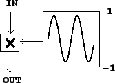
This gives us a technique for shifting the component frequencies of a sound, called ring modulation, which is shown in its simplest form in Figure 5.2. An oscillator provides a carrier signal, which is simply multiplied by the input. In this context the input is called the modulating signal. The term ``ring modulation" is often used more generally to mean multiplying any two signals together, but here we'll just consider using a sinusoidal carrier signal. (The technique of ring modulation dates from the analog era [Str95]; digital multipliers now replace both the VCA (Section 1.5) and the ring modulator.)
Figure 5.3 shows a variety of results
that may be obtained by multiplying a (modulating) sinusoid of
angular frequency ![]() and peak amplitude
and peak amplitude
![]() , by a (carrier) sinusoid of angular
frequency
, by a (carrier) sinusoid of angular
frequency ![]() and peak amplitude 1:
and peak amplitude 1:
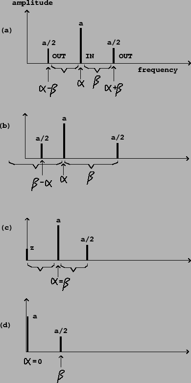 |
Parts (a) and (b) of the figure show ``general" cases where
![]() and
and ![]() are nonzero and
different from each other. The component frequencies of the output
are
are nonzero and
different from each other. The component frequencies of the output
are
![]() and
and
![]() . In part (b), since
. In part (b), since
![]() , we get a negative
frequency component. Since cosine is an even function, we
have
, we get a negative
frequency component. Since cosine is an even function, we
have
In the special case where
![]() , the second (difference)
sideband has zero frequency. In this case phase will be significant
so we rewrite the product with explicit phases, replacing
, the second (difference)
sideband has zero frequency. In this case phase will be significant
so we rewrite the product with explicit phases, replacing
![]() by
by ![]() , to
get:
, to
get:
Finally, part (d) shows a carrier signal whose frequency is
zero. Its value is the constant ![]() (not
(not ![]() ;
zero frequency is a special case). Here we get only one sideband,
of amplitude
;
zero frequency is a special case). Here we get only one sideband,
of amplitude ![]() as usual.
as usual.
We can use the distributive rule for multiplication to find out
what happens when we multiply signals together which consist of
more than one partial each. For example, in the situation above we
can replace the signal of frequency ![]() with a
sum of several sinusoids, such as:
with a
sum of several sinusoids, such as:
Figure 5.4 shows the result of
multiplying a complex periodic signal (with several components
tuned in the ratio 0:1:2:![]() ) by a sinusoid. Both
the spectral envelope and the component frequencies of the result
are changed according to relatively simple rules.
) by a sinusoid. Both
the spectral envelope and the component frequencies of the result
are changed according to relatively simple rules.
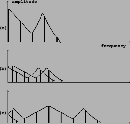 |
The resulting spectrum is essentially the original spectrum combined with its reflection about the vertical axis. This combined spectrum is then shifted to the right by the carrier frequency. Finally, if any components of the shifted spectrum are still left of the vertical axis, they are reflected about it to make positive frequencies again.
In part (b) of the figure, the carrier frequency (the frequency of the sinusoid) is below the fundamental frequency of the complex signal. In this case the shifting is by a relatively small distance, so that re-folding the spectrum at the end almost places the two halves on top of each other. The result is a spectral envelope roughly the same as the original (although half as high) and a spectrum twice as dense.
A special case, not shown, is to use a carrier frequency half
the fundamental. In this case, pairs of partials will fall on top
of each other, and will have the ratios 1/2 : 3/2 : 5/2
:![]() to give an odd-partial-only signal an
octave below the original. This is a very simple and effective
octave divider for a harmonic signal, assuming you know or can find
its fundamental frequency. If you want even partials as well as odd
ones (for the octave-down signal), simply mix the original signal
with the modulated one.
to give an odd-partial-only signal an
octave below the original. This is a very simple and effective
octave divider for a harmonic signal, assuming you know or can find
its fundamental frequency. If you want even partials as well as odd
ones (for the octave-down signal), simply mix the original signal
with the modulated one.
Part (c) of the figure shows the effect of using a modulating frequency much higher than the fundamental frequency of the complex signal. Here the unfolding effect is much more clearly visible (only one partial, the leftmost one, had to be reflected to make its frequency positive). The spectral envelope is now widely displaced from the original; this displacement is often a more strongly audible effect than the relocation of partials.
As another special case, the carrier frequency may be a multiple of the fundamental of the complex periodic signal; then the partials all land back on other partials of the same fundamental, and the only effect is the shift in spectral envelope.