We have heretofore discussed digital audio signals as if they
were capable of describing any function of time, in the sense that
knowing the values the function takes on the integers should
somehow determine the values it takes between them. This isn't
really true. For instance, suppose some function ![]() (defined for real numbers) happens to attain the value 1 at all
integers:
(defined for real numbers) happens to attain the value 1 at all
integers: ![]() for
for
![]() . We might guess
that
. We might guess
that ![]() for all real
for all real ![]() . But
perhaps
. But
perhaps ![]() happens to be one for integers and zero
everywhere else--that's a perfectly good function too, and nothing
about the function's values at the integers distinguishes it from
the simpler
happens to be one for integers and zero
everywhere else--that's a perfectly good function too, and nothing
about the function's values at the integers distinguishes it from
the simpler ![]() . But intuition tells us that the
constant function is in the spirit of digital audio signals,
whereas the one that hides a secret between the samples isn't. A
function that is ``possible to sample" should be one for which we
can use some reasonable interpolation scheme to deduce its values
for non-integers from its values for integers.
. But intuition tells us that the
constant function is in the spirit of digital audio signals,
whereas the one that hides a secret between the samples isn't. A
function that is ``possible to sample" should be one for which we
can use some reasonable interpolation scheme to deduce its values
for non-integers from its values for integers.
It is customary at this point in discussions of computer music
to invoke the famous Nyquist
theorem. This states (roughly speaking) that if a function is a
finite or even infinite combination of REAL SINUSOIDS, none of
whose angular frequencies exceeds ![]() , then,
theoretically at least, it is fully determined by the function's
values on the integers. One possible way of reconstructing the
function would be as a limit of higher- and higher-order polynomial
interpolation.
, then,
theoretically at least, it is fully determined by the function's
values on the integers. One possible way of reconstructing the
function would be as a limit of higher- and higher-order polynomial
interpolation.
The angular frequency ![]() , called the Nyquist
frequency, corresponds to
, called the Nyquist
frequency, corresponds to ![]() cycles per second
if
cycles per second
if ![]() is the sample rate. The corresponding period
is two samples. The Nyquist frequency is the best we can do in the
sense that any real sinusoid of higher frequency is equal, at the
integers, to one whose frequency is lower than the Nyquist, and it
is this lower frequency that will get reconstructed by the ideal
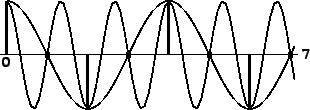
interpolation process. For instance, a REAL SINUSOID with angular
frequency between
is the sample rate. The corresponding period
is two samples. The Nyquist frequency is the best we can do in the
sense that any real sinusoid of higher frequency is equal, at the
integers, to one whose frequency is lower than the Nyquist, and it
is this lower frequency that will get reconstructed by the ideal
interpolation process. For instance, a REAL SINUSOID with angular
frequency between ![]() and
and ![]() , say
, say ![]() , can be written
as
, can be written
as
 |
We conclude that when, for instance, we're computing an EXPLICIT
SUM OF SINUSOIDS, either as a wavetable or as a real-time signal,
we had better drop any sinusoid in the sum whose frequency exceeds
![]() . But the picture in general is not this
simple, since most techniques other than additive synthesis don't
lead to neat, band-limited signals (ones whose components stop at
some limited frequency.) For example, a sawtooth wave of frequency
. But the picture in general is not this
simple, since most techniques other than additive synthesis don't
lead to neat, band-limited signals (ones whose components stop at
some limited frequency.) For example, a sawtooth wave of frequency
![]() , of the form put out by Pd's
, of the form put out by Pd's
![]() object but considered as
a continuous function
object but considered as
a continuous function ![]() , expands to:
, expands to:
Many synthesis techniques, even if not strictly band-limited,
give partials which may be made to drop off more rapidly than
![]() as in the sawtooth example, and are thus
more forgiving to work with digitally. In any case, it is always a
good idea to keep the possibility of foldover in mind, and to train
your ears to recognize it.
as in the sawtooth example, and are thus
more forgiving to work with digitally. In any case, it is always a
good idea to keep the possibility of foldover in mind, and to train
your ears to recognize it.
The first line of defense against foldover is simply to use high sample rates; it is a good practice to systematically use the highest sample rate that your computer can easily handle. The highest practical rate will vary according to whether you are working in real time or not, CPU time and memory constraints, and/or input and output hardware, and sometimes even software-imposed limitations.
A very non-technical treatment of sampling theory is given in [Bal03]. More detail can be found in [Mat69, pp. 1-30].