So far we have dealt with audio signals, which are just
sequences ![]() defined for integers
defined for integers ![]() ,
which correspond to regularly spaced points in time. This is often
an adequate framework for describing synthesis techniques, but real
electronic music applications usually also entail other
computations which have to be made at irregular points in time. In
this section we'll develop a framework for describing what we will
call control computations. We
will always require that any computation correspond to a specific
logical time. The logical time
controls which sample of audio output will be the first to reflect
the result of the computation.
,
which correspond to regularly spaced points in time. This is often
an adequate framework for describing synthesis techniques, but real
electronic music applications usually also entail other
computations which have to be made at irregular points in time. In
this section we'll develop a framework for describing what we will
call control computations. We
will always require that any computation correspond to a specific
logical time. The logical time
controls which sample of audio output will be the first to reflect
the result of the computation.
In a non-real-time system such as Csound, this means that logical time proceeds from zero to the length of the output soundfile. Each "score card" has an associated logical time (the time in the score), and is acted upon once the audio computation has reached that time. So audio and control calculations (grinding out the samples and handling note cards) are each handled in turn, all in increasing order of logical time.
In a real-time system, logical time, which still corresponds to the time of the next affected sample of audio output, is always slightly in advance of real time, which is measured by the sample that is actually leaving the computer. Control and audio computations still are carried out in alternation, sorted by logical time.
The reason for using logical time and not real time in computer music computations is to keep the calculations independent of the actual execution time of the computer, which can vary for a variety of reasons, even for two seemingly identical calculations. When we are calculating a new value of an audio signal or processing some control input, real time may pass but we require that the logical time stay the same through the whole calculation, as if it took place instantaneously. As a result of this, electronic music computations, if done correctly, are deterministic: two runs of the same real-time or non-real-time audio computation, each having the same inputs, should have identical results.
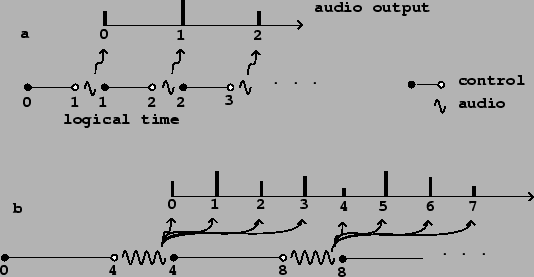 |
Figure 3.2 part (a) shows schematically how logical time and sample computation are lined up. Audio samples are computed periodically (as shown with wavy lines), but before the calculation of each sample we do all the control calculations (marked as straight line segments). First we do the control computations associated with logical times starting at zero, up to but not including one; then we compute the first audio sample (of index zero), at logical time one. We then do all control calculations up to but not including logical time 2, then the sample of index one, and so on. (Here we are adopting certain conventions about labeling that could be chosen differently. For instance, there is no fundamental reason control should be pictured as coming ``before" audio computation but it is easier to think that way.)
Part (b) of the figure shows the situation if we wish to compute
the audio output in blocks of more than one sample at a time. Using
the variable ![]() to denote the number of elements in a
block (so
to denote the number of elements in a
block (so ![]() in the figure), the first audio
computation will output samples
in the figure), the first audio
computation will output samples ![]() all at
once in a block. We have to do the relevant control computations
for all four periods of time in advance. There is a delay of
all at
once in a block. We have to do the relevant control computations
for all four periods of time in advance. There is a delay of
![]() samples between logical time and the
appearance of audio output.
samples between logical time and the
appearance of audio output.
Audio is computed in blocks in Max/MSP, Csound and Pd, and sample by sample in SuperCollider. The reason for computing by blocks is to increase the efficiency of unit generators (Csound) or tilde objects (Pd; Max/MSP). Each tilde object incurs overhead each time it is called, equal to perhaps twenty times the cost of computing one sample on average. If the block size is one, this means an overhead of 2,000%; if it is sixty-four (as in Pd), the overhead is only some 30%.
SuperCollider overcomes this problem by compiling signal processing algorithms into machine language, thus avoiding the efficiency problem of the other environments described here. The main drawback to this scheme is the additional software development effort required, and the greater difficulty of maintaining the program. This is also perhaps the main reason SuperCollider only runs on one machine architecture; to adapt it to others will require re-writing the machine code generator.