Waveshaping

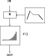
Another approach to modulating a signal, called waveshaping, is simply to pass it through a suitably chosen nonlinear function. A block diagram for doing this is shown in Figure 5.5. The function $f()$ (called the transfer function) distorts the incoming waveform into a different shape. The new shape depends on the shape of the incoming wave, on the transfer function, and finally on the amplitude of the incoming signal. Since the amplitude of the input waveform affects the shape of the output waveform (and hence the timbre), this gives us an easy way to make a continuously varying family of timbres, simply by varying the input level of the transformation. For this reason, it is customary to include a leading amplitude control as part of the waveshaping operation, as shown in the block diagram.

Figure 5.5: Block diagram for waveshaping an input signal using a nonlinear function $f()$. An amplitude adjustment step precedes the function lookup, to take advantage of the different effect of the wavetable lookup at different amplitudes.

The amplitude of the sinusoid is called the waveshaping index. In many situations a small index leads to relatively little distortion (hence a more nearly sinusoidal output) and a larger one gives a more distorted, hence richer, timbre.

Figure 5.6 shows a familiar example of waveshaping, in which the $f()$ amounts to a clipping function. This example shows clearly how the input amplitude--the index--can affect the output waveform. The clipping function passes its input to the output unchanged as long as it stays in the interval between -0.3 and +0.3. So when the input (in this case a sinusoid) does not exceed 0.3 in absolute value, the output is the same as the input. But when the input grows past the 0.3 limit, it is limited to 0.3; and as the amplitude of the signal increases the effect of this clipping action is progressively more severe. In the figure, the input is a decaying sinusoid. The output evolves from a nearly square waveform at the beginning to a pure sinusoid at the end. This effect will be well known to anyone who has played an instrument through an overdriven amplifier. The louder the input, the more distorted will be the output. For this reason, waveshaping is also sometimes called distortion.

Figure 5.6: Clipping as an example of waveshaping. The input (a) is a sinusoid of varying amplitude, and the waveshaping function (b) clips its input to the interval between -0.3 and +0.3. The output is shown in (c).

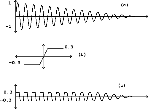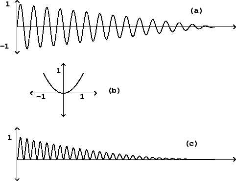
Figure 5.7 shows a much simpler and easiest to analyse situation, in which the transfer function simply squares the input:

$$f(x) = {x^2}$$

For a sinusoidal input,

$$x[n] = a \cos(\omega n + \phi)$$

we get

$$f(x[n]) = {{a^2} \over 2} \left ( 1 + \cos(2 \omega n + 2 \phi) \right )$$

If the amplitude $a$ equals one, this just amounts to ring modulating the sinusoid by a sinusoid of the same frequency, whose result we described in the previous section: the output is a CD signal plus a signal at twice the original frequency. However, unlike the case of ring modulation, the amplitude of the output grows as the square of the input.

Figure 5.7: Waveshaping using a quadratic transfer function $f(x) = {x^2}$. The input (a) yields an output (c) at twice the frequency.

Keeping the same transfer function, we now consider the effect of sending in a combination of two sinusoids with amplitudes $a$ and $b$, and angular frequencies $\alpha$ and $\beta$. For simplicity, we'll omit the initial phase terms. We set:

$$x[n] = a \cos(\alpha n) + b \cos(\beta n)$$

and plugging this into $f$ gives

$$f(x[n]) = {{a^2} \over 2} \left ( 1 + \cos(2 \alpha n) \right )$$

$$+ {{b^2} \over 2} \left ( 1 + \cos(2 \beta n) \right )$$

$$+ a b \left ( \cos ( (\alpha + \beta) n ) + \cos ( (\alpha - \beta) n ) \right )$$

The first two terms are just what we would get by sending the two sinusoids through separately. The third term is the product of the two input terms, which comes from the middle, cross term in the expansion,

$$f(x+y) = {x^2} + 2 x y + {y^2}$$

This effect, called intermodulation, becomes more and more dominant as the number of terms in the input increases; if there are $k$ sinusoids in the input there are only $k$ ``straight" terms in the product, but there are $({k^2}-k)/2$ intermodulation terms.

As compared to ring modulation, which is linear in its input, waveshaping is nonlinear. While we were able to analyze linear processes by considering their action separately on all the components of the input, in this nonlinear case we also have to consider the interactions between components. The results are far more complex--sometimes sonically much richer, but, on the other hand, harder to understand or predict.

In general, we can show that a periodic input, no matter how complex, will give an output of the same periodicity. If the period is $\tau$ so that

$$x[n + \tau] = x[n]$$

then we immediately get

$$f(x[n+\tau]) = f(x[n]) .$$

Combinations of periodic tones at consonant intervals give rise to distortion products at subharmonics. For instance, if two periodic signals $x$ and $y$ are a musical fourth apart (periods in the ratio 4:3), then the sum of the two repeats at the lower rate given by the common subharmonic. In equations we would have:

$$x[t + \tau/3] = x[t]$$

$$y[t + \tau/4] = y[t]$$

which implies

$$x[t + \tau] + y[t+\tau] = x[t] + y[t]$$

and so the distorted sum $f(x+y)$ would repeat after a period of $\tau$:

$$f(x+y)[n + \tau] = f(x+y)[n].$$

This has been experienced by every electric guitarist who has set the amplifier to ``overdrive" and played the open B and high E strings together: the distortion product is pitched the same as the low E string, two octaves below the high one.

To get a somewhat more explicit analysis of the effect of waveshaping on an incoming signal, it is sometimes useful to write the function $f$ as a finite or infinite polynomial series:

$$f(x) = {f_0} + {f_1}x + {f_2}{x^2} + {f_3}{x^3} + \cdots$$

If the input signal $x[n]$ is a sinusoid $a \cos(\omega n)$, we can consider the action of the above terms separately:

$$f(x[n]) = {f_0} + a {f_1}\cos(\omega n) + {a^2} {f_2} {\cos^2} (\omega n) + {a^3} {f_3} {\cos^3} (\omega n) + \cdots$$

Since the higher order terms are multiplied by higher powers of the amplitude $a$, a lower value of $a$ will weight the earlier terms more heavily, and a higher value will make the higher-order terms more prominent.

The individual terms' spectra can be found by applying the cosine product formula repeatedly:

$$1 = \cos (0)$$

$$x[n] = \cos (\omega n)$$

$${x^2}[n] = {1 \over 2} + {1 \over 2} \cos (2\omega n)$$

$${x^3}[n] = {1 \over 4} \cos (-\omega n) + {2 \over 4} \cos (\omega n) + {1 \over 4} \cos (3 \omega n)$$

$${x^4}[n] = {1 \over 8} \cos (-2\omega n) + {3 \over 8} \cos... ... {3 \over 8} \cos (2 \omega n) + {1 \over 8} \cos (4 \omega n)$$

$${x^5}[n] = {1 \over 16} \cos (-3\omega n) + {4 \over 16} \c... ... \over 16} \cos (3 \omega n) + {1 \over 16} \cos (5 \omega n)$$

and so on. The relative weights of the components will be recognized as Pascal's triangle. They can be approximated by a Gaussian curve whose width, for the $x^k$ term of the expansion, grows as the square root of $k$.

The negative-frequency terms (which have been shown separately here for clarity) are to be combined with the positive ones; the spectral envelope is folded into itself in the same way as in the ring modulation example of Figure Figure 5.4.

As long as the coefficients $f_k$ are all positive numbers or zero, then so are all the amplitudes of the sinusoids in the expansions above. In this case all the phases stay coherent as $a$ varies and so we get a widening of the spectrum (and possibly a drastically increasing amplitude) with increasing values of $a$. On the other hand, if some of the $f_k$ are positve and others negative, the different expansions will interfere destructively; this will give a more complicated-sounding spectral evolution.

Note also that the successive expansions all contain only even or only odd partials. If the transfer function (in series form) happens to contain only even powers:

$$f(x) = {f_0} + {f_2}{x^2} + {f_4}{x^4} + \cdots$$

then the result, having only even partials, will sound an octave higher than the incoming sinusoid. If only odd powers show up in the expansion of $f(x)$, then the output will contain only odd partials. Even if $f$ can't be expressed exactly as a power series (for example, the clipping function of Figure 5.3), it is still true that if $f$ is an even function, i.e., if

$$f(-x) = f(x)$$

you will get only even harmonics and if $f$ is an odd function,

$$f(-x) = -f(x)$$

you get odd harmonics.

Many mathematical tricks have been proposed to use waveshaping to generate specified spectra. It turns out that you can generate pure sinusoids at any harmonic of the fundamental by using a Chebyshef polynomial as a transfer function [Leb79], and from there you can go on to build any desired static spectrum. Generating families of spectra by waveshaping a sinusoid of variable amplitude turns out to be trickier, although several interesting special cases have been found, one of which is developed here in chapter [].