


It is sometimes desirable to connect the outputs of one or more delays in a network back into their own or each others' inputs. Instead of getting one or several echos of the original sound as in the simple example above, we can potentially get an infinite number of echos, each one feeding back into the network to engender yet others.
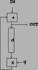
The simplest example of a recirculating network is the recirculating comb filter whose block
diagram is shown in Figure 7.7.
As with the earlier, simple comb filter, the input signal is sent
down a delay line whose length is  samples.
Unlike the simple comb filter, the delay line's output is also
inserted back in its input; the delay's input is now the sum of the
original input and the delay output. The output is multiplied by a
number
samples.
Unlike the simple comb filter, the delay line's output is also
inserted back in its input; the delay's input is now the sum of the
original input and the delay output. The output is multiplied by a
number  before feeding it back into its input.
 |
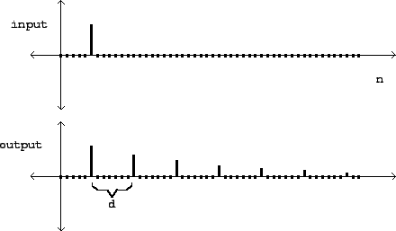
The time domain behavior of the recirculating comb filter is
shown in Figure 7.8. Here we
consider the effect of sending an impulse into the network. We get
back the original impulse, plus a series of echos, each in turn
samples after the previous one, and
multiplied each time by the gain .
Note that we have chosen a gain that is less
than one in absolute value. If we chose a gain greater than one (or
less than -1), each echo would have a larger magnitude than the
previous one. Instead of falling exponentially as they do in the
figure, they would grow exponentially. A recirculating network
whose output eventually falls toward zero after its input
terminates is called stable;
one whose output grows without bound is called unstable.
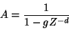
We can also analyse the recirculating comb filter in the frequency domain. The situation is now complicated enough that it is almost prohibitively hard to analyze using real sinusoids, and so we get the first real payoff for having introduced complex numbers, which greatly simplify the analysis.
If, as before, we feed the input with the signal,
![\begin{displaymath} X[n] = Z^n \end{displaymath}](img723.png)
 , we can write the output as
![\begin{displaymath} Y[n] = (1 + g{Z^{-d}} + {g^2}{Z^{-2d}} + \cdots) X[n] \end{displaymath}](img724.png)

 to
give:
to
give:
 ,
,
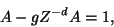
A faster (but slightly less intuitive) method to get the same
result is to examine the recirculating network itself to yield an
equation for , as follows. Since we named the input
![$X[n]$](img685.png) and the output
and the output ![$Y[n]$](img730.png) , the
signal going into the delay line is
, the
signal going into the delay line is ![$X[n]+Y[n]$](img731.png) , and
passing this through the delay line and multiplier gives
, and
passing this through the delay line and multiplier gives
![\begin{displaymath} (X[n]+Y[n])g{Z^{-d}} \end{displaymath}](img732.png)
![\begin{displaymath} Y[n] = (X[n]+Y[n])g{Z^{-d}} \end{displaymath}](img733.png) and using
and using ![$A=Y[n]/X[n]$](img734.png) gives:
gives: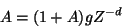 .
.
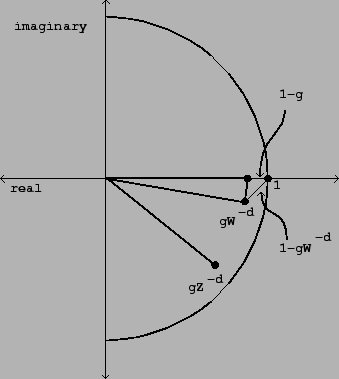
Now we would like to make a graph of the gain as a function of
frequency, as we did for non-recirculating comb filters in Figure
7.6. This again requires that we
make a preliminary picture in the complex plane. We would like to
estimate the magnitude of equal to:
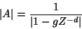
 is the reciprocal of the length of the segment
reaching from the point 1 to the point .
Figure 7.10 shows a graph of the
frequency response as a function of
the angular frequency
is the reciprocal of the length of the segment
reaching from the point 1 to the point .
Figure 7.10 shows a graph of the
frequency response as a function of
the angular frequency
 .
.
 |
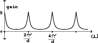 |
Figure 7.9 can be used to
analyze how the frequency response
should behave qualitatively as a function of .
The height and bandwidth of the peaks both depend on . The maximum value the can
attain is when

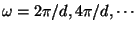 as in the
simple comb filter above. At these maxima it reaches
as in the
simple comb filter above. At these maxima it reaches
The next important question is the bandwidth of the peaks in the
frequency response. So we would like to find a particular
frequency,
 , giving rise to a value of
that is, say, 3 decibels below
the maximum. To do this, we return to Figure 7.9, and try to find
, giving rise to a value of
that is, say, 3 decibels below
the maximum. To do this, we return to Figure 7.9, and try to find  so that the distance from the point 1 to the point

 times the distance from 1 to
(since :1 is a ratio
of approximately 3 decibels).
times the distance from 1 to
(since :1 is a ratio
of approximately 3 decibels).
We do this by arranging for the imaginary part of  to be roughly
  or its negative,
making a nearly isosocles right triangle between the points 1,
, and . (Here we're
supposing that is at least 2/3 or so; otherwise
this approximation isn't very good). The hypoteneuse of a right
isococles triangle is always times the
leg, and so the gain drops by that factor compared to its
maximum.
or its negative,
making a nearly isosocles right triangle between the points 1,
, and . (Here we're
supposing that is at least 2/3 or so; otherwise
this approximation isn't very good). The hypoteneuse of a right
isococles triangle is always times the
leg, and so the gain drops by that factor compared to its
maximum.
We now make another approximation, that the imaginary part of
is approximately the angle in radians
it cuts from the real axis:

 approaches its
maximum value of
approaches its
maximum value of  . .
. .
As with the non-recirculating comb filter of section 7.3, the teeth of the comb are
closer together for larger valuse of the delay .
On the other hand, a delay of  (the shortest
possible) gets only one tooth (at zero frequency) below the Nyquist
frequency
(the shortest
possible) gets only one tooth (at zero frequency) below the Nyquist
frequency  (the next tooth, at
  , corresponds again to a frequency of zero by
foldover).
, corresponds again to a frequency of zero by
foldover).
So the recirculating comb filter with is
just a low-pass filter. Delay networks with one-sample delays will
be the basis for designing many other kinds of digital filters in
chapter ![[*]](file:/usr/share/latex2html/icons/crossref.png) .
.
 . The frequency
 . The peak gain is
  = 5. Peaks are
much narrower than for the simple comb filter.
= 5. Peaks are
much narrower than for the simple comb filter.