Impulse responses of recirculating filters

In Section 7.4 we derived the impulse response of a recirculating comb filter, of which the one-pole low-pass filter is a special case. In Figure 8.22 we show the result for two low-pass filters and one complex one-pole resonant filter. All are elementary recirculating filters as introduced in section 8.2.3. Each is normalized to have unit maximum gain.

In the case of a low-pass filter, the impulse response gets longer (and lower) as the pole gets closer to one. Suppose the pole is at a point $1-1/n$ (so that the cutoff frequency is $1/n$ radians). The normalizing factor is also $1/n$. After $n$ points, the output diminishes by a factor of

$${ {\left ( 1-{1\over n} \right ) } ^ n } \approx {1\over e}$$

where $e$ is Euler's constant, about 2.718. The filter can be said to have a settling time of $n$ samples. In the figure, $n=5$ for part (a) and $n=10$ for part (b). In general, the settling time (in samples) is approximately one over the cutoff frequency (in angular units).

Figure 8.22: The impulse response of three elementary recirculating (one-pole) filters, normalized for peak gain 1: (a) low-pass with $P=0.8$; (b) low-pass with $P=0.9$; (c) band-pass, with $\vert P\vert=0.9$ and a center frequency of $2\pi /10$.

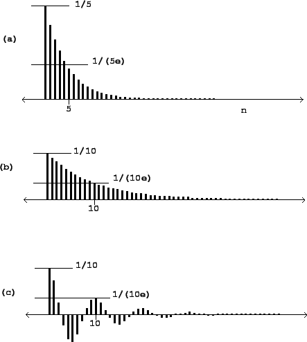The situation gets more interesting when we look at a resonant one-pole filter, that is, one whose pole lies off the real axis. In part (c) of the figure, the pole $P$ has absolute value 0.9 (as in part (b)), but its argument is set to $2\pi /10$ radians. We get the same settling time as in part (b), but the output rings at the resonant frequency (and so at a period of 10 samples in this example).

A natural question to ask is, how many periods of ringing do we get before the filter decays to strength $1/e$? If the pole of a resonant has modulus $1-1/n$ as above, we have seen in section 8.2.3 that the bandwidth (call it $b$) is about $1/n$, and we have seen here that the settling time is about $n$. The resonant frequency (call it $\omega$) is the argument of the pole, and the period in samples is $2 \pi / \omega$. The number of periods that make up the settling time is thus:

$${{n} \over {2\pi/\omega}} = {{1} \over {2\pi}} {{\omega} \over {b}} = {{q} \over {2\pi}}$$

where $q$ is the quality of the filter, defined as the center frequency divided by bandwidth. Resonant filters are often specified in terms of the center frequency and ``q", instead of bandwidth.