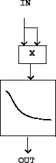
It is frequently desirable to use the time-varying power of an incoming signal to trigger or control a musical process. To do this, we will need a procedure for measuring the power of an audio signal. Since most audio signals pass through zero many times per second, it won't suffice to take the absolute value of the signal as a measure if its power, instead, we must make an average of the power over an interval of time long enough that its oscillations won't whow up in the power estimate, but short enough that changes in signal level are quickly reflected in the power estimate. A computation that provides a timely, time-varying power estimate is called an envelope follower.
The output of a low-pass filter can be viewed as a moving
average of its input. For example, suppose we apply a normalized
one-pole low-pass filter (as in Figure 8.21) to an incoming signal ![]() . The output (call it y[n]) is the sum of the delay output
times
. The output (call it y[n]) is the sum of the delay output
times ![]() (real-valued for a low-pass filter), with
(real-valued for a low-pass filter), with
![]() times the input:
times the input:
For more insight into the design of a suitable low-pass filter
for an envelope follower, we analyze it from the point of view of
signal spectra. If, for instance, we put in a real-valued
sinusoid:
The situation for a signal with several components is similar.
Suppose the input signal is now,
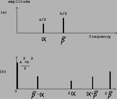 |
Envelope followers may also be used on noisy signals, which may be thought of as signals with dense spectra. In this situation there will be difference frequencies arbitrarily close to zero frequency, and filtering them out entirely will be impossible; we will always get fluctuations in the output, but they will decrease proportionally as the filter's pass band is narrowed.
Although a narrower bass band will always give a cleaner output, whether for discrete or continuous spectra, the filter's settling time will lengthen proportionally as the bass band is narrowed. There is thus a tradeoff between getting a quick response and a smooth result.