


Next: Examples Up: Modulation Previous:
Waveshaping Contents
Index
Frequency and phase modulation
If a sinusoid is given a frequency which varies slowly in time
we hear it as having a varying pitch. But if the pitch changes so
quickly that our ears can't track the change--for instance, if the
change itself occurs at or above the fundamental frequency of the
sinusoid--we hear a timbral change. The timbres so generated are
rich and widely varying. The discovery by John Chowning of this
possibility [Cho73]
revolutionized the field of computer music. Here we develop
frequency modulation, usually called FM,
as a special case of waveshaping [Leb79]; the treatment here is adapted
from an earlier publication [Puc01].
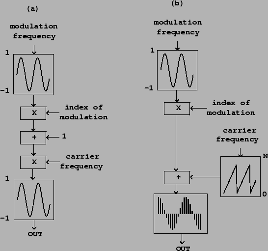
The FM technique, in its simplest form, is shown in figure
5.8 part (a). A frequency-modulated
sinusoid is one whose frequency varies sinusoidally, at some
angular frequency  , about a central
frequency
, about a central
frequency  , so that the instantaneous
frequencies vary between
, so that the instantaneous
frequencies vary between  and
and
 , with parameters controlling the frequency of variation, and
 controlling the depth of variation. The
parameters , , and
are called the carrier frequency, the modulation frequency, and the index of modulation, respectively.
controlling the depth of variation. The
parameters , , and
are called the carrier frequency, the modulation frequency, and the index of modulation, respectively.
It is customary to use a simpler, essentially equivalent
formulation in which the phase, instead of the frequency, of the
carrier sinusoid is modulated sinusoidally. (This gives an
equivalent result since the instantaneous frequency is just the
change of phase, and since the sample-to-sample change in a
sinusoid is just another sinusoid.) The phase modulation
formulation is shown in part (b) of the figure. If the carrier and
modulation frequencies don't themselves vary in time, the resulting
signal can be written as
The parameter  , which takes the place of the earlier
parameter , is also called the index of
mosulation; it too controls the extent of frequency variation
relative to the carrier frequency . If
, which takes the place of the earlier
parameter , is also called the index of
mosulation; it too controls the extent of frequency variation
relative to the carrier frequency . If
 , there is no frequency variation and the
expression reduces to the unmodified, carrier sinusoid:
, there is no frequency variation and the
expression reduces to the unmodified, carrier sinusoid:
Figure 5.8: Block diagram
for frequency modulation (FM) synthesis: (a) the classic form; (b)
realized as phase modulation.
 |
To analyse the resulting spectrum we can write,
so we can consider it as a sum of two waveshaping generators, each
operating on a sinusoid of frequency and
with a waveshaping index , and each ring modulated with
a sinusoid of frequency . The waveshaping
function  is given by
 for the first term and by
 for the second.
Returning to Figure 5.4, we
can see at a glance what the spectrum will look like. The two
harmonic spectra, of the waveshaping outputs
and
have, respectively, harmonics tuned to
and
and each is multiplied by a sinusoid at the carrier frequency. So
there will be a spectrum centered at the carrier frequency
, with sidebands at both even and odd
multiples of the modulation frequency ,
contributed respectively by the sine and cosine waveshaping terms
above. The index of modulation , as it changes,
controls the relative strength of the various partials. The
partials themselves are situated at the frequencies
where
As with any situation where two periodic signals are multiplied, if
there is some common supermultiple of the two periods, the
resulting product will repeat at that longer period. So if the two
periods are  and
and  , where
 and
and  are relatively
prime, they both repeat after a time interval of
are relatively
prime, they both repeat after a time interval of  . In other words, if the two have frequencies which are
both multiples of some common frequency, so that
. In other words, if the two have frequencies which are
both multiples of some common frequency, so that
 and
and
 , again with
and relatively prime, the result will repeat at
a frequency of the common submultiple
, again with
and relatively prime, the result will repeat at
a frequency of the common submultiple  . On the
other hand, of no common submultiple can be
found, or if the only submultiples are lower than any discernable
pitch, then the result will be inharmonic.
. On the
other hand, of no common submultiple can be
found, or if the only submultiples are lower than any discernable
pitch, then the result will be inharmonic.
Much more about FM can be found in textbooks [Moo90, p. 316] [DJ85] [Bou00] and research publications;
some of the possibilities are shown in the following examples.
Next: Examples Up: Modulation Previous:
Waveshaping Contents
Index
Miller Puckette 2006-03-03