Waveshaping using an exponential function

We return now to the spectra computed on Page , corresponding to waveshaping functions of the form $f(x) = x^k$. We note with pleasure that not only are they all in phase (so that they can be superposed with easily predictable results) but also that the spectra spread out increasingly with $k$. Also, in a series of the form,

$$f(x) = {f_0} + {f_1} x + {f_2} {x^2} + \cdots,$$

a higher index of modulation will lend more relative weight to the higher power terms in the expansion; as we saw seen earlier, if the index of modulation is $a$, the terms are $x^k$ multiplied by $f_0$, $af_1$, ${a^2}{f_2}$, and so on.

To take the simplest possible example, suppose we wish $f_0$ to be the largest term for $0<a<1$, then for it to be overtaken by the more quickly growing $af_1$ term for $1<a<2$, which is then overtaken by the ${a^2}{f_2}$ term for $2<a<3$ and so on, so that the $n$th term takes over at an index equal to $n$. To make this happen we just require that

$${a_1} = {a_0} , 2 {a_2} = {a_1}, 3 {a_3} = {a_2} , \cdots$$

and so fixing $a_0$ at 1, we get ${a_1}=1$, ${a_2}=1/2$, ${a_3}=1/6$, and in general,

$${a_k} = {1 \over {(1 \cdot 2 \cdot 3 \cdot \cdots \cdot k}}$$

These are just the coefficients for the power series for the function

$$f(x) = {e ^ x}$$

where $e \approx 2.7$ is Euler's constant.

Before plugging in $e^x$ as a transfer function it's wise to plan how we will deal with signal amplitude, since $e^x$ grows quickly as a function of $x$. If we're going to plug in a sinusoid of amplitude $a$, the maximum output will be $e^a$, occuring whenever the phase is zero. A simple and natural choice is simply to divide by $e^a$ to reduce the peak to one, giving:

$${{f(a \cos(\omega n))} \over {e^a}} = {e^{a (\cos(\omega n) - 1)}}$$

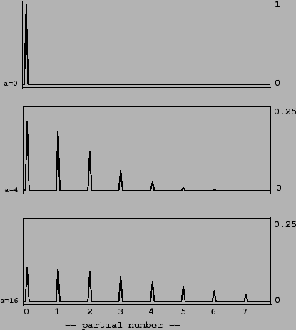
This is realized in Patch E06.exponential.pd. Resulting spectra for $a=$ 0, 4, and 16 are shown in Figure 5.13. As the waveshaping index rises, progressively less energy is present in the fundamental; the energy is increasingly spread over the partials.

Figure 5.13: Spectra of waveshaping output using an exponential transfer function. Indices of modulation of 0, 4, and 16 are shown; note the different vertical scales.