Sinusoids, amplitude and frequency

Electronic music is made by synthesizing or processing digital audio signals. These are sequences of numbers,

$$..., x[n-1], x[n], x[n+1], ...$$

where the index $n$, called the sample number, may range over some or all the integers. A single number in the sequence is called a sample. (Some writers use the word ``sample" differently, to mean ``recorded sound"--but in this book we'll only use the word to mean a single number.) An example of a digital audio signal is the Sinusoid:

Sinusoid

$$x[n] = a \cos (\omega n + \phi )$$

where $a$ is the amplitude, $\omega$ is the angular frequency, and $\phi$ is the initial phase. The phase is a function of the sample number $n$, equal to $\phi + \omega n$. The initial phase is the phase at the zeroth sample ($n=0$).

Strictly speaking, this is the real Sinusoid, distinct from the complex Sinusoid introduced later in chapter 7; but where there's no chance of confusion we will simply say ``Sinusoid" to speak of the real-valued one.

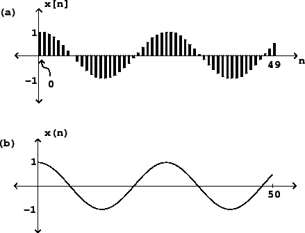
Figure 1.1 shows a Sinusoid graphically. In part (a) of the figure, the horizontal axis shows successive values of $n$ and the vertical axis shows the corresponsding values of $x[n]$. The graph is drawn in such a way as to emphasize the sampled nature of the signal. Alternatively, we could draw it more simply as a continuous curve (part b). The upper drawing is the most faithful representation of the (digital audio) Sinusoid, whereas the lower one can be considered as idealization of it.

Figure 1.1: A digital audio signal, showing its discrete-time nature (part a), and idealized as a continuous function (part b). This signal is a (real-valued) Sinusoid, fifty points long, with amplitude 1, angular frequency 0.24, and initial phase zero.

Sinusoids play a key role in audio processing because, if you shift one of them left or right by any number of samples, you get another one. This makes it easy to calculate the effect of all sorts of operations on sinusoids. Our ears use this same special property to help us parse incoming sounds, which is why sinusoids, and combinations of sinusoids, can be used for a variety of musical effects.

Digital audio signals do not have any intrinsic relationship with time, but to listen to them we must choose a sample rate, usually given the variable name $R$, which is the number of samples that fit into a second. Time is related to sample number by $Rt = n$, or $t = n/R$. A sinusoidal signal with angular frequency $\omega$ has a real-time frequency equal to

$$f = {{\omega R} \over {2 \pi}}$$

in cycles per second, because a cycle is $2\pi$ radians and a second is $R$ samples.

A real-world audio signal's amplitude might be expressed as a time-varying voltage or air pressure, but the samples of a digital audio signal are unitless numbers. We'll casually assume here that there is ample numerical accuracy so that we can ignore round-off errors, and that the numerical format is unlimited in range, so that samples may take any value we wish. However, most digital audio hardware works only over a fixed range of input and output values, most often between -1 and 1. Modern digital audio processing software usually uses a floating-point representation for signals. This allows us to use whatever units are most convenient for any given task, as long as the final audio output is within the hardware's range.